UMAP and XY
A Landscape can show cells in a low dimensional embedding, such as a UMAP, as well as in tissue. A UMAP places cells with similar expression near each other, so islands of cells suggest cell types and states. XY plots each cell's expression of two genes against each other.
For single-cell data, a linked Clustergram complements the UMAP with a higher-dimensional view. The UMAP shows how cells relate to each other; the Clustergram shows which genes distinguish them, either as cluster signatures, such as marker-gene dot plots, or as single-cell expression across a selected group of cells. The Chromium PBMC tutorial shows both.
Switching between tissue and UMAP
When the data include a UMAP, such as adata.obsm["X_umap"] passed with spatial
DegaFiles, UMAP and SPATIAL move the same cells between their embedding
and their positions in the tissue. The move is animated, so you can follow a
group of cells from one view to the other.
Kidney cells move from the tissue into their UMAP and back. The image returns when the cells are back in place.
Cluster selections carry over between views: select a cluster in the UMAP, and switch to SPATIAL to see where those cells are in the tissue. In UMAP and XY, unselected cells are dimmed rather than hidden.
Single-cell Landscapes from AnnData Zarr
A single-cell Landscape, without spatial data, reads an AnnData Zarr store directly in the browser. It opens in the UMAP; there is no SPATIAL or IMG view.
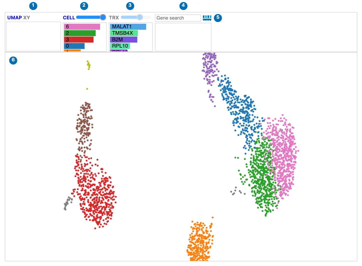
PBMC 3k cells in a UMAP, colored by Leiden cluster.
| Control | What it does | |
|---|---|---|
| 1 | UMAP · XY | Switch between the UMAP and the two-gene XY view. |
| 2 | CELL | Cell size, and the clusters of the cells in view. |
| 3 | TRX | The genes, and whether their values are whole-dataset or estimated for the view; see below. |
| 4 | Gene search | Color cells by one or more genes. |
| 5 | Celldega logo | Opens the Landscape documentation. |
| 6 | The view | Scroll to zoom, drag to pan, hover for details, and click to select. |
Search for a gene to color the cells by its expression:
Searching for LYZ highlights the monocytes; larger cells and stronger expression opacity make the pattern easier to see.
To prepare a store, add a CSC copy of a sparse expression layer so the browser can read one gene at a time. The example uses raw counts:
import zarr

adata.layers["counts_csc"] = adata.layers["counts"].tocsc()
adata.write_zarr("cells.zarr")
zarr.consolidate_metadata("cells.zarr")

landscape = dega.viz.Landscape(
    zarr_url="cells.zarr",
    zarr_layer="counts_csc",
    cluster_attr="cell_type",
    cell_attr=["cell_type", "sample_id"],
    nbhd_edit=True,
)
zarr_url accepts an HTTP(S) URL or a local store under the working directory,
which Python serves over HTTP. The browser loads metadata and obsm["X_umap"]
from the store, then reads requested genes with Zarrita. Dense or CSR expression
needs a CSC copy; zarr_layer selects it explicitly. An optional adata
supplies overriding cell metadata, cluster colors, and UMAP positions; its cell
IDs must match the store. See
AnnData Zarr storage
for gene statistics, layer discovery, and format details.
Viewport cell types and estimated expression
Panning or zooming in a UMAP or XY view updates the CELL bars with the number of cells of each type in view, as the spatial view does when zoomed in. Points are sized in embedding units, so they grow as you zoom in.
The gene bars follow the view too, and the TRX button's color shows what they hold:
- Blue: every cell is in view, so the bars show whole-dataset values.
- Purple: zoomed in, the bars show estimates from cell-type signatures.
- Gray: zoomed in without matching signatures, so the bars keep the whole-dataset values.
Hover over TRX for an explanation of the current state. In UMAP and XY, TRX is an indicator: clicking it does not load anything.
Zooming into the Tabula Sapiens atlas: the CELL bars count the cell types in view, and TRX turns purple as the gene bars become signature estimates.
What the estimate means
For each gene, the estimate is the number of visible cells of each type times that type's mean expression, summed and divided by the number of visible cells:
estimated mean(gene) = Σ (visible cells of a type × the type's mean expression) / visible cells
For example, if the view holds 80 T cells with a mean of 10 for a gene and 20 B cells with a mean of 0, the estimate is 8. If those particular T cells actually average 20, the estimate is still 8: it captures which cell types are in view, not variation within a type. No per-cell expression is downloaded when the view changes. Gene coloring and XY axes always use actual cell expression.
For exact expression of every gene, or a Clustergram of the cells in view, draw a neighborhood around them and use the matching cell-level AnnData in Python:
selected = landscape.get_selected_cells(adata)
if selected.n_obs:
    mat = dega.clust.Matrix(selected)
    mat.filter("row", by="var", num=min(500, selected.n_vars))
    mat.cluster()
    cgm = dega.viz.Clustergram(matrix=mat)
Providing signatures
Estimates need each cell type's mean expression, grouped the same way as the cells being shown:
adata_sig: an AnnData of means, sent with the widget.gene_signature_url: a separate signature AnnData Zarr, read by the browser; better for large signatures (tens of MB).- Spatial DegaFiles use their own
df_sig.parquet, each default cluster's mean counts per cell, only while the Landscape shows the DegaFiles' own clusters. Passing anadatareplaces the cell metadata, so then provideadata_sigorgene_signature_urlinstead.
Prepare signatures with Scanpy
Give Landscape each cell type's mean expression, as an AnnData with cell
types as obs_names and genes as var_names. Use layers["counts"] for
mean raw counts per cell when the Landscape colors cells from raw counts. An
optional log1p layer can hold mean log-normalized expression. For a
cell-level AnnData with raw counts in layers["counts"] and log1p in X:
import scanpy as sc

signature = sc.get.aggregate(adata, by="cell_type", func="mean", layer="counts")
signature.layers["counts"] = signature.layers.pop("mean")
signature.layers["log1p"] = sc.get.aggregate(adata, by="cell_type", func="mean").layers["mean"]
signature.uns["viewport_signature"] = {
    "groupby": "cell_type",
    "layers": {"counts": "mean counts per cell", "log1p": "mean log1p counts per 10,000"},
}

landscape = dega.viz.Landscape(
    zarr_url="cells.zarr",
    cluster_attr="cell_type",
    adata_sig=signature,
    nbhd_edit=True,
)
Larger signatures are better saved as a separate AnnData Zarr:
import json
import zarr

signature.uns["viewport_signature"] = json.dumps(signature.uns["viewport_signature"])
signature.write_zarr("cell_type_signatures.zarr")
zarr.consolidate_metadata("cell_type_signatures.zarr")

landscape = dega.viz.Landscape(
    zarr_url="cells.zarr",
    cluster_attr="cell_type",
    gene_signature_url="cell_type_signatures.zarr",
)
Means must be finite and nonnegative. Signature Zarr stores require a dense
matrix; adata_sig also accepts sparse means. The estimate reads
viewport_signature["layer"] when set, else layers["counts"], else X;
other units, such as mean log1p, also work and are named in TRX's tooltip.
Match the layer to the expression that colors the cells. When a dataset
mixes UMI counts with read counts (for example 10x and Smart-seq2), use
library-size-normalized log1p expression and the signatures' log1p layer
("layer": "log1p"). groupby names the cell attribute the labels come
from (default: cluster_attr). Every visible cell must have a matching
signature; otherwise the gene bars keep the whole dataset (TRX gray) and
TRX's tooltip reports the coverage. Up to 200 genes are shown.
XY: two-gene expression
XY initializes X and Y with the two genes with the highest whole-dataset mean
expression, unless you supply xy_genes. Ties retain dataset gene order; missing
statistics fall back to that order after genes with known means. A dataset with
one gene initializes X only. Changing or restoring the axes keeps your choices.
XY plots each cell's expression of two genes, with LIN (linear) and
LOG (log1p) axes. It is available for spatial and single-cell data with
gene expression, even without a UMAP. Type the genes in the X and Y
boxes, or select two genes before clicking XY. The XY view is still being
developed.
landscape.set_xy("CD3D", "MS4A1", scale="log1p")
landscape.landscape_state = "spatial"  # or "umap" when available
UMAP's second coordinate increases upward, matching the usual AnnData and Scanpy orientation; so does XY's Y axis.
Widget: Python-backed interactions
landscape.landscape_statereports and sets the view:"spatial","umap", or"xy".landscape.xy_genesandlandscape.xy_scalehold the XY axes.- Gates drawn in UMAP or XY select cells; read them with
landscape.get_selected_cells(adata). See Neighborhoods.
Source code
Screenshot sources
Animations and screenshots show the
Atera kidney
DegaFiles with its AnnData's UMAP, the PBMC 3k AnnData Zarr store from the
Chromium PBMC tutorial,
and the Tabula Sapiens atlas
(Tabula Sapiens Consortium, via CZ CELLxGENE Discover, CC BY 4.0). They were
captured with Celldega 0.28.0 using
scripts/docs_screenshots/capture.py.