Visualize Your Own Data
This guide follows a public 10x Genomics Xenium human pancreas dataset from the instrument's output to linked views of your own analysis: your clusters over the tissue and in a UMAP, a marker-gene dot plot, and gene-set enrichment. The same steps apply to your own Xenium data. Run the code in a Jupyter or marimo notebook.
 Xenium output bundle
   │
   ├─ 1. pre.main ──► DegaFiles ──────────────┐
   │                                          ▼
   └─ 2. Scanpy ────► AnnData ──────────► 3. Landscape: clusters, UMAP
                         │                    ▲
                         │                    │ 5. linked
                         └─► 4. Matrix ─► Clustergram ─► Enrich
Each step's output for this dataset is already hosted, so you can start at any step. To explore the prepared data before installing anything, try the Quick Start.
1. Prepare DegaFiles from the instrument output
DegaFiles arrange the images, cells, transcripts, and expression so that the
browser can load only what is in view. Preprocessing needs the pre extra and
a native libvips installation:
pip install "celldega[pre]"
Download the Xenium output bundle from the 10x Genomics dataset page (a 5.7 GB zip), and unpack it:
mkdir -p data/xenium && cd data/xenium
curl -LO https://cf.10xgenomics.com/samples/xenium/2.0.0/Xenium_V1_human_Pancreas_FFPE/Xenium_V1_human_Pancreas_FFPE_outs.zip
unzip Xenium_V1_human_Pancreas_FFPE_outs.zip -d Xenium_V1_human_Pancreas_FFPE_outs
Then write the DegaFiles:
import celldega as dega

dega.pre.main(
    sample="Xenium_V1_human_Pancreas_FFPE_outs",
    data_root_dir="data/xenium",
    path_dega_files="data/DegaFiles/pancreas",
    tile_size=250,
    image_tile_layer="all",
)
pre.main handles Xenium (including Atera) and MERSCOPE bundles; see the
Atera preprocessing example.
To view the DegaFiles, serve their directory over HTTP and pass the URL to a
Landscape:
port = dega.viz.get_local_server(file_server_root="data/DegaFiles/pancreas")
landscape = dega.viz.Landscape(base_url=f"http://localhost:{port}")
landscape
To share them, upload the directory to GitHub, Hugging Face, or a cloud bucket; see Host and share prepared data. The rest of this guide uses the hosted DegaFiles for this dataset:
base_url = (
    "https://raw.githubusercontent.com/broadinstitute/celldega_Xenium_human_Pancreas_FFPE/"
    "main/Landscape_Xenium_V1_human_Pancreas_FFPE_outs_webp"
)
2. Analyze with Scanpy
Read the cell-by-gene counts from the same output bundle, then cluster as usual with Scanpy:
import scanpy as sc

outs = "data/xenium/Xenium_V1_human_Pancreas_FFPE_outs"
adata = sc.read_10x_h5(f"{outs}/cell_feature_matrix.h5")
adata.layers["counts"] = adata.X.copy()

sc.pp.filter_cells(adata, min_counts=10)
sc.pp.filter_genes(adata, min_cells=5)
sc.pp.normalize_total(adata)
sc.pp.log1p(adata)
sc.pp.pca(adata)
sc.pp.neighbors(adata)
sc.tl.umap(adata)
sc.tl.leiden(adata, flavor="igraph", n_iterations=2, directed=False)
This takes about two minutes for the 122,678 cells that pass the filter.
Celldega links your analysis to the DegaFiles by cell ID: read_10x_h5
names cells by their Xenium cell IDs (such as aaaadnje-1), the same IDs the
DegaFiles use. If you read the data another way, such as with
spatialdata-io, set
adata.obs_names = adata.obs["cell_id"].astype(str) first.
3. See your clusters in the tissue
Pass the AnnData to the Landscape. Cells take your Leiden clusters and colors, and the UMAP becomes available with the UMAP button:
landscape = dega.viz.Landscape(base_url=base_url, adata=adata, cluster_attr="leiden")
landscape
Select a cluster in the UMAP, then switch to SPATIAL to see where those cells are in the tissue; see Spaces and embeddings, which shows this dataset's islet cells moving between the two views.
4. Find marker genes with a dot-plot Clustergram
Rank each cluster's marker genes, then summarize the cells by cluster. In the dot plot, color is a gene's mean expression in a cluster, scaled across clusters, and dot size is the fraction of the cluster's cells that express it:
import celldega as dega

sc.tl.rank_genes_groups(adata, groupby="leiden")

markers = dega.clust.Matrix(adata, groupby="leiden")
markers.filter_by_size(0.05)  # genes detected in at least 5% of a cluster's cells
markers.norm("row", by="zscore")
markers.cluster(view="rank_genes_groups", levels=[1, 3, 5, 10])

cgm = dega.viz.Clustergram(matrix=markers, rank_dim=3)
cgm
cluster(view=..., levels=...) precomputes views with 1, 3, 5, and 10 marker
genes per cluster; the DIM slider moves between them, and rank_dim=3 opens
at three markers per cluster. See Clustergram
for every interaction.
5. Link the views and interpret with Enrich
Link the Landscape and Clustergram, and add Enrich to look up the selected genes in public gene-set libraries:
dega.viz.spatial_clustergram(landscape, cgm, enrich=True)
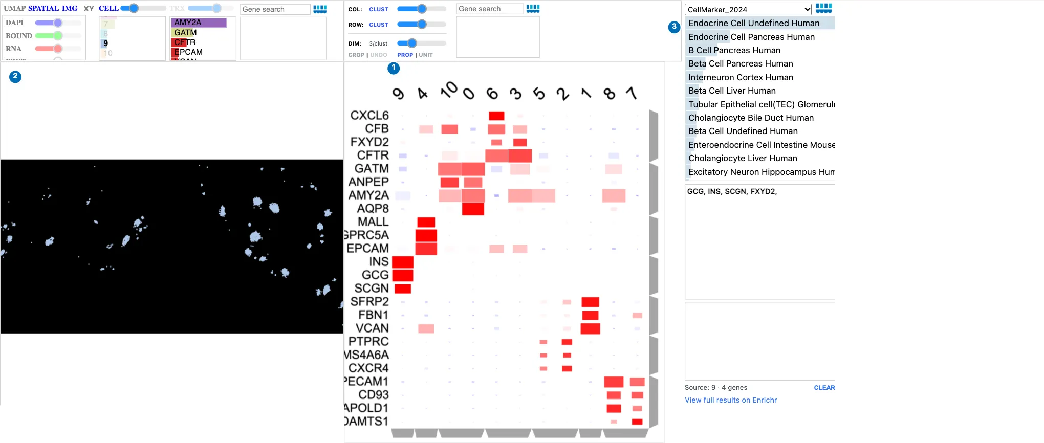
Clicking the islet cluster's column (9 here) in the Clustergram.
| What happened | |
|---|---|
| 1 | Clicking the cluster's column label selected it. Its markers, INS, GCG, and SCGN, mark insulin- and glucagon-producing islet cells. |
| 2 | The Landscape shows only that cluster's cells: the islets, scattered through the pancreas. |
| 3 | Enrich received the cluster's top marker genes and ranks endocrine and beta cell gene sets first. |
Clicking a gene's row label colors the cells by that gene, and a row dendrogram branch sends a group of genes to Enrich. Your Leiden numbers may differ from this example's. See Landscape–Clustergram–Enrich for more linked workflows.
6. Save and share
Save the clustered dot plot so that it reopens without recomputing, in Python or in a web page:
markers.write_zarr("pancreas_markers.zarr")
restored = dega.clust.Matrix.read_zarr("pancreas_markers.zarr")
A notebook saved with its widget state can be published as an interactive report, as the example notebooks on this site are; see two ways to use a visualization.
Next steps
- From Scanpy & Squidpy: what Celldega reads from your AnnData, and how to bring selections and annotations back into it.
- Visualizations: every interaction in Landscape, Clustergram, and the other views.
- Neighborhoods: draw regions, such as islets, and summarize the cells inside them.
- Scanpy–Squidpy Xenium pancreas tutorial: add Squidpy's spatial neighborhood enrichment.
- Chromium PBMC tutorial: the same steps for single-cell data, which need no DegaFiles.
Screenshot sources
The screenshot shows the hosted pancreas DegaFiles with the
hosted Scanpy AnnData
for this dataset, captured with Celldega 0.28.0 using
scripts/docs_screenshots/capture.py.
The code on this page was run with Celldega 0.28.0 on the 10x output bundle.
Data: 10x Genomics, FFPE Human Pancreas with Xenium Multimodal Cell Segmentation.