Explore perturbation clusters

To find perturbations with similar profiles, start with the browsable Matches tables. These show the top 100 most correlated/anticorrelated matches per perturbation rather than the full all-vs-all matrix.

For comparisons outside those matches, the full cosine-similarity matrices are available on Zenodo and mirrored on Cell Painting Gallery. Here we query the CRISPR matrix to compare three perturbations without loading the entire matrix into memory.

from random import choices, seed

import matplotlib.pyplot as plt
import polars as pl
import seaborn as sns

We use a versioned Cell Painting Gallery mirror of the Zenodo release for reproducibility and faster HTTP range reads. Polars can read the metadata and selected columns without downloading the full 239 MB file. Avoid calling head().collect() on the full-width matrix: even a few rows would request all 7,977 columns.

The stored values are cosine similarities: 1 means profiles point in the same direction, 0 means they are orthogonal, and -1 means they point in opposite directions. Cosine distance, if needed, is 1 - similarity.

ZENODO_RECORD_ID = "20496083"
CPG_BASE = (
    "https://cellpainting-gallery.s3.amazonaws.com/"
    "cpg0016-jump/source_all/workspace/publication_data/jump_rr"
)
similarities = pl.scan_parquet(
    f"{CPG_BASE}/{ZENODO_RECORD_ID}/crispr_cosinesim_full.parquet/content"
)

Columns are JUMP IDs (JCP2022_X), and rows follow the same order. See the metadata tutorial for mapping these IDs to gene names. We select three perturbations, then collect only their columns and matching rows.

seed(42)
cols = similarities.collect_schema().names()
ncols = len(cols)
sampled_col_idx = sorted(choices(range(ncols), k=3))
sampled_cols = [cols[ix] for ix in sampled_col_idx]

sampled_similarities = (
    similarities.select(sampled_cols)
    .with_row_index()
    .filter(pl.col("index").is_in(sampled_col_idx))
    .drop("index")
    .collect()
)
sampled_similarities

shape: (3, 3)

JCP2022_805125	JCP2022_802572	JCP2022_801315
f32	f32	f32
1.0	0.01572	0.066012
0.01572	1.0	0.12222
0.066012	0.12222	1.0

Finally, we plot them in a heatmap for easier visualisation

pandas_similarity = sampled_similarities.to_pandas()
pandas_similarity.index = pandas_similarity.columns
sns.heatmap(
    pandas_similarity,
    annot=True,
    fmt=".3f",
    vmin=-1,
    vmax=1,
    center=0,
    cmap=sns.color_palette("vlag", as_cmap=True),
    cbar_kws={"label": "Cosine similarity"},
)
plt.yticks(rotation=30)
plt.tight_layout()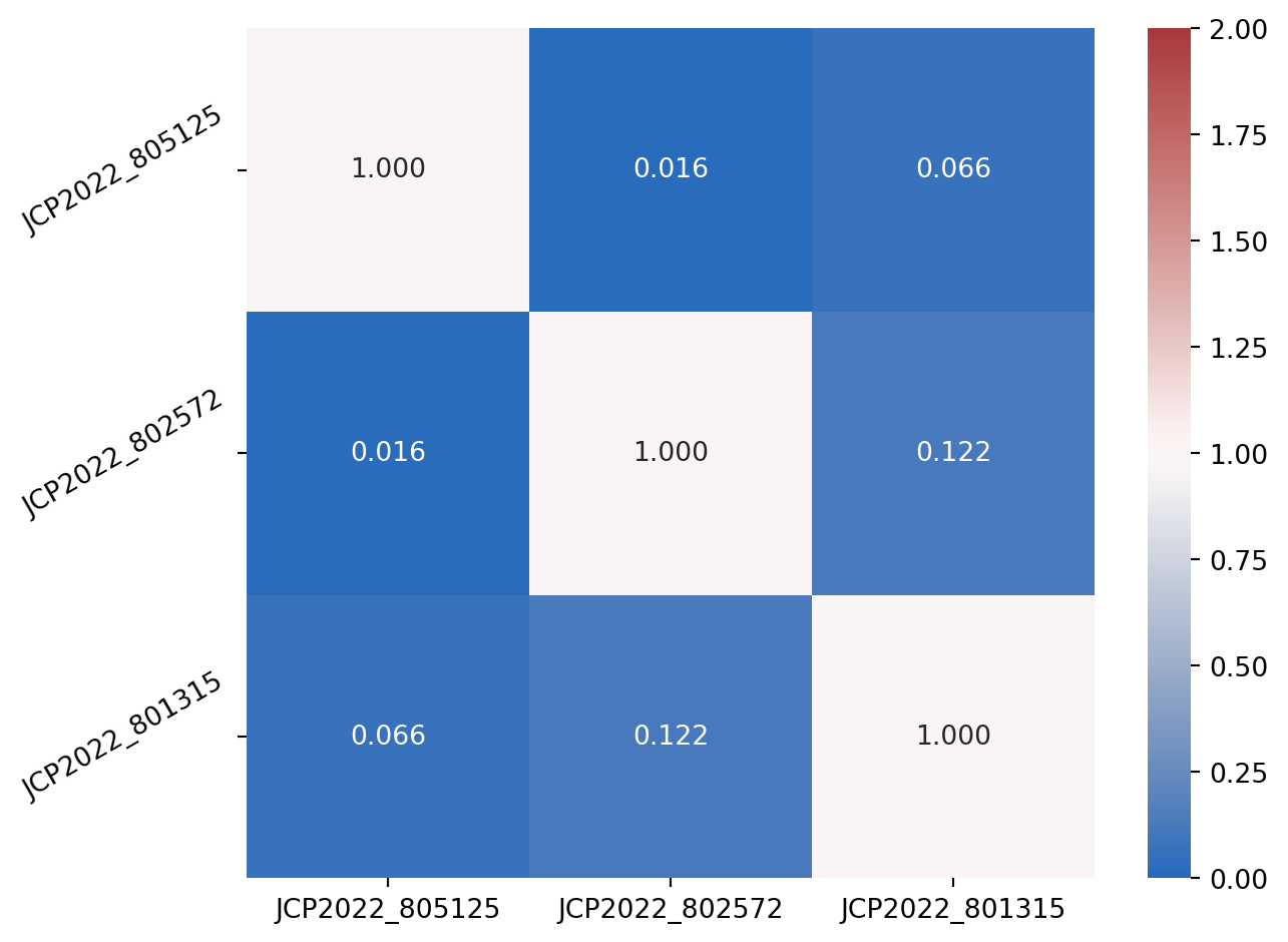

Off-diagonal entries compare different perturbations; the diagonal shows self-similarity (approximately 1). This example illustrates querying selected pairs, not a biological clustering analysis.

Other Formats