Display perturbation images

This notebook demonstrates how to retrieve and plot all channels for one site using the jump_portrait library.

import duckdb
import matplotlib.colors as mpl  # noqa: CPY001
import numpy as np
from jump_portrait.fetch import get_item_location_metadata, get_jump_image
from matplotlib import pyplot as plt

#

First, we need to get location information telling us where all images corresponding to a specific perturbation can be found. We will use the “get_item_location” function from jump_portrait for this. Here we retrieve image locations for the “RAB30” gene:

gene_info = get_item_location_metadata("RAB30")
gene_info.shape

Downloading data from 'https://github.com/jump-cellpainting/datasets/raw/c68deb2babc83747e6b14d8a77e5655138a6086a/metadata/well.csv.gz' to file '/home/runner/.cache/pooch/4efbf4dd3dd9aaecc8ccb9fc3c6b4122-well.csv.gz'.
Downloading data from 'https://zenodo.org/api/records/18729301/files/jump_index.parquet/content' to file '/home/runner/.cache/pooch/de9363bf9723d94feff1a5d15d111dbe-content'.

(90, 12)

There are 90 images: 9 sites/well X 5 replicate wells X 2 data types (CRISPR & ORF). We can also retrieve locations for compound data. By default, the function assumes a query by INCHI key. We can also query by JCP ID by specifying the query column:

cmpd_info_byinchi = get_item_location_metadata("CLETVKMYAXARPO-UHFFFAOYSA-N")
cmpd_info_byjcp = get_item_location_metadata("JCP2022_011844", input_column="JCP2022")

print(cmpd_info_byinchi.shape)
print(cmpd_info_byjcp.shape)

(34, 12)
(34, 12)

There are 34 sites corresponding to this compound. We’ve written a function to display all channels for a specific image. Note that this is just one possible way to display images - we’ve included the function here so that you can modify it to suit your own needs.

def display_site(
    source: str,
    batch: str,
    plate: str,
    well: str,
    site: int,
    label: str,
    int_percentile: float,
) -> None:
    """Plot all channels from one image.

    Parameters
    ----------
    source : String
        Source ID for image of interest.
    batch : String
        Batch ID for image of interest.
    plate : String
        Plate ID for image of interest.
    well : String
        Well ID for image of interest.
    site : String
        Site ID for image of interest.
    label : String
        Label to display in lower left corner.
    int_percentile: float
        Rescale the image from 0 - this percentile of intensity values.

    """
    n_rows = 2
    n_cols = 3

    # Make images
    axes = plt.subplots(n_rows, n_cols, figsize=(2.6 * n_cols, 2.6 * n_rows))[1]
    axes = axes.ravel()

    channel_rgb = {
        "AGP": "#FF7F00",  # Orange
        "DNA": "#0000FF",  # Blue
        "ER": "#00FF00",  # Green
        "Mito": "#FF0000",  # Red
        "RNA": "#FFFF00",  # Yellow
    }

    for ax, (channel, rgb) in zip(axes, channel_rgb.items()):
        cmap = mpl.LinearSegmentedColormap.from_list(channel, ("#000", rgb))

        img = get_jump_image(source, batch, plate, well, channel, site)

        ax.imshow(img, vmin=0, vmax=np.percentile(img, int_percentile), cmap=cmap)
        ax.axis("off")

        # Add channel name label in the top left corner
        ax.text(
            0.05,
            0.95,
            channel,
            horizontalalignment="left",
            verticalalignment="top",
            fontsize=18,
            color="black",
            bbox=dict(
                facecolor="white", alpha=0.8, edgecolor="none", boxstyle="round,pad=0.3"
            ),
            transform=ax.transAxes,
        )

    # put label in last subplot
    ax = axes[-1]
    ax.text(
        0.5,
        0.5,
        label,
        horizontalalignment="center",
        verticalalignment="center",
        fontsize=20,
        color="black",
        transform=ax.transAxes,
    )
    ax.axis("off")

    # show plot
    plt.tight_layout()

We can get the required location parameters from the location info that we retrieved earlier. We transform the first row from pyarow format to Python. Here we get parameters for the first site in the JCP compound results:

with duckdb.connect() as con:
    meta_dict = (
        con.sql(
            "SELECT COLUMNS('Metadata_(Source|Batch|Plate|Well|Site)') FROM cmpd_info_byjcp"
        )
        .to_arrow_table()
        .to_batches()[0]
        .to_pylist()[0]
    )
    (
        source,
        batch,
        plate,
        well,
        site,
    ) = [
        meta_dict[f"Metadata_{k}"] for k in ("Source", "Batch", "Plate", "Well", "Site")
    ]

# cmpd_info_byjcp.select(
#     pl.col(f"Metadata_{x}" for x in ("Source", "Batch", "Plate", "Well", "Site"))
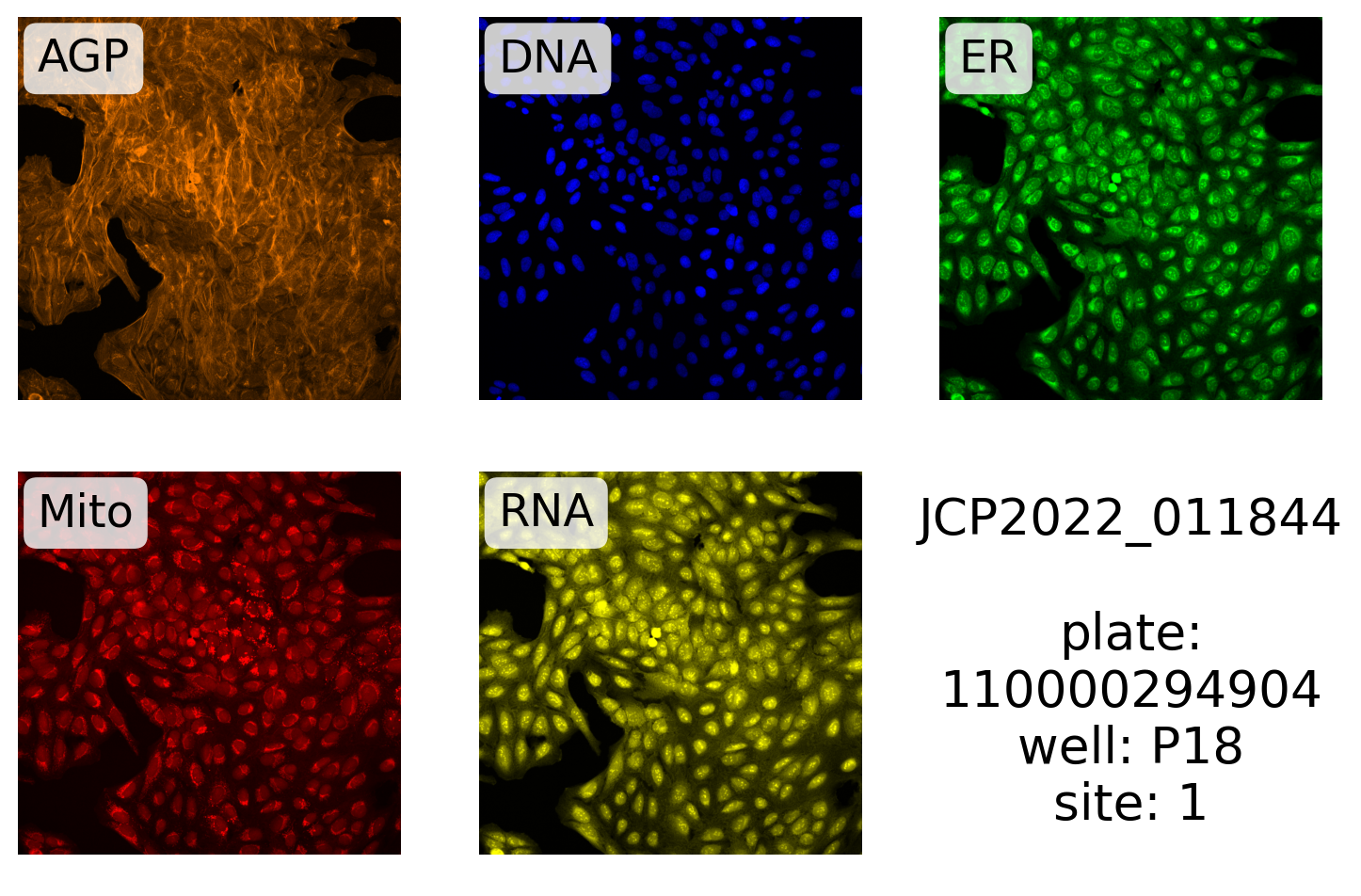
# ).row(0)

Next, we define the label and make the plot:

label = "{}\n\nplate:\n{}\nwell: {}\nsite: {}"

display_site(
    source,
    batch,
    plate,
    well,
    site,
    label.format("JCP2022_011844", plate, well, site),
    99.5,
)

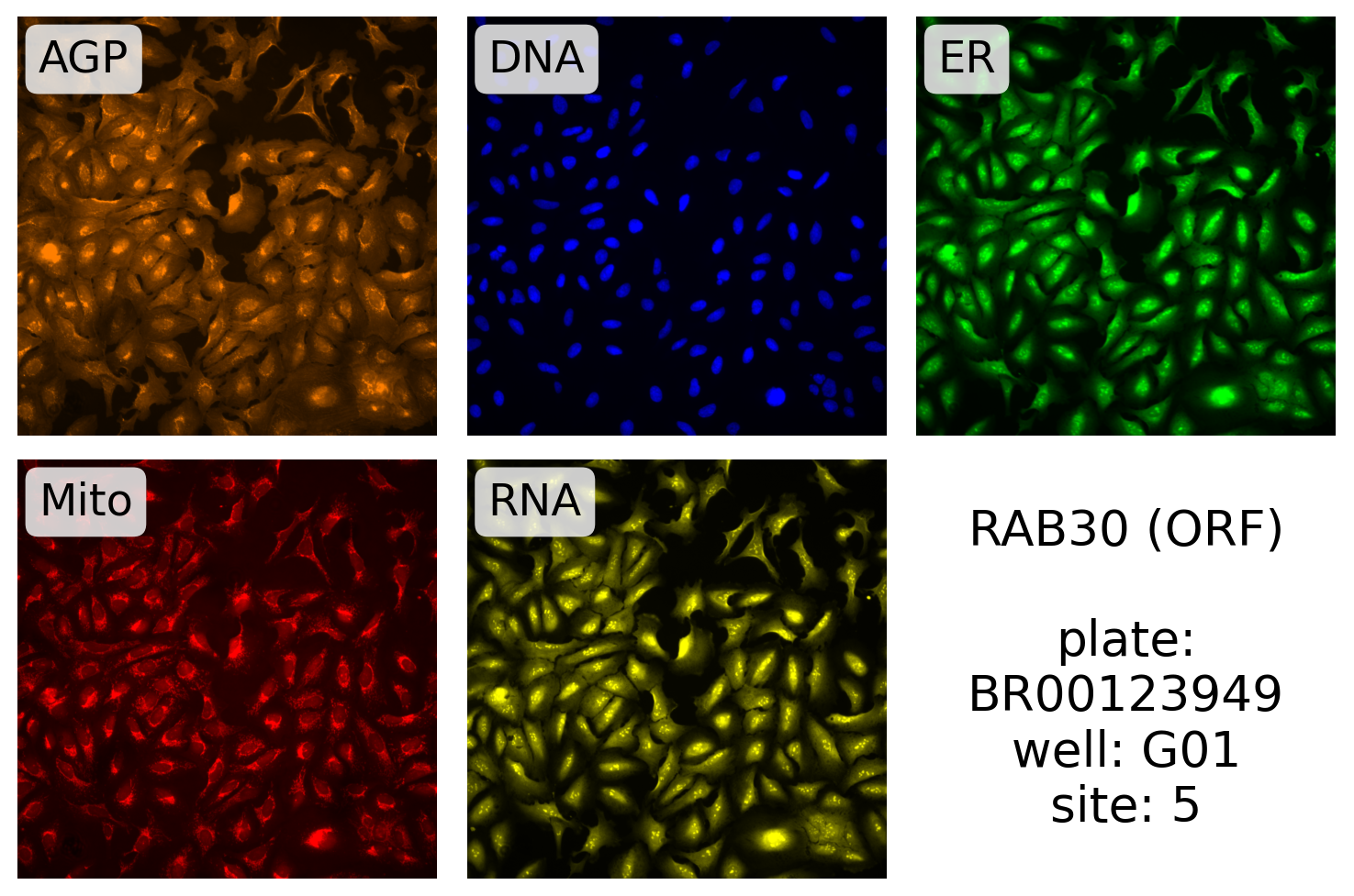
Here, we plot one of the RAB30 ORF images (ORF JCP ids start with 9):

with duckdb.connect() as con:
    meta_dict = (
        con.sql("FROM gene_info WHERE Metadata_JCP2022.starts_with('JCP2022_9')")
        .to_arrow_table()
        .to_batches()[0]
        .to_pylist()[0]
    )
source, batch, plate, well, site = [
    meta_dict[f"Metadata_{x}"] for x in ("Source", "Batch", "Plate", "Well", "Site")
]
display_site(
    source,
    batch,
    plate,
    well,
    site,
    label.format("RAB30 (ORF)", plate, well, site),
    99.5,
)

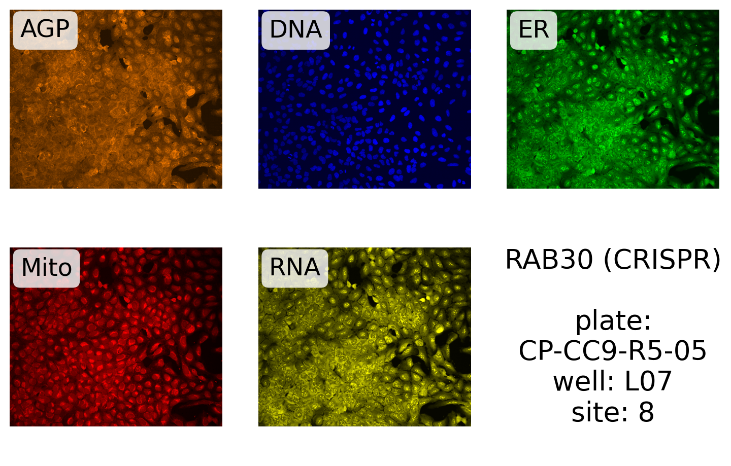
And for CRISPR (The JCP ID number starts with 8):

with duckdb.connect() as con:
    meta_dict = (
        con.sql("FROM gene_info WHERE Metadata_JCP2022.starts_with('JCP2022_8')")
        .to_arrow_table()
        .to_batches()[0]
        .to_pylist()[0]
    )
source, batch, plate, well, site = [
    meta_dict[f"Metadata_{x}"] for x in ("Source", "Batch", "Plate", "Well", "Site")
]

display_site(
    source,
    batch,
    plate,
    well,
    site,
    label.format("RAB30 (CRISPR)", plate, well, site),
    99.5,
)

Other Formats