Explore perturbation clusters

A common question we aim to ask is “What other perturbations look like mine?” The easiest way to get the answer for this question is using our browsable datasets. In this case we would like to use the ‘Matches’ databases, which provide cosines similarities between perturbations within a dataset, obtained from all-vs-all calculations.

The limitation of this approach is that the size of JUMP results in two challenges: - Calculating the distances across all pairs of perturbations is intractable for most computers without a GPU (Graphics Processing Unit). - The resultant similarity matrix is too big for web browser-based exploration, so we limit the browsable similarity dataset to the top 100 most correlated/anticorrelated pairs of perturbations.

Despite the aforementioned problems, we provide the full matrix of perturbation distances in case it is of use to data analysts. You can find this and other datasets on Zenodo. The data files of interest for this exercise are “{org,crispr}_cosinesim_full.parquet”.

The following analysis focuses on showcasing how to query one of these distance matrices to find all the distances between any given perturbation and all others. One use-case of this is testing how similar perturbation A and B are relative to perturbation C’s similarity to A.

import requests
from random import choices, seed

import matplotlib.pyplot as plt
import polars as pl
import seaborn as sns

We select the CRISPR dataset for this example. As with previous examples, this is a lazy-loaded data frame. This enables us to download very big datasets without worrying about whether or not they will fill into memory. In these datasets, the values range between 0 and 2, where 0 means that two profiles are the same, 1 means that they are orthogonal (completely uncorrelated) and 2 means that they are completely anticorrelated.

latest_id = requests.get(
    "https://zenodo.org/api/records/15029005/versions/latest"
).json()["id"]
distances = pl.scan_parquet(
    f"https://zenodo.org/api/records/{latest_id}/files/crispr_cosinesim_full.parquet/content"
)
distances.head().collect()

shape: (5, 7_977)

JCP2022_800002	JCP2022_804257	JCP2022_800001	JCP2022_807659	JCP2022_804265	JCP2022_806265	JCP2022_806261	JCP2022_806729	JCP2022_803314	JCP2022_802979	JCP2022_806962	JCP2022_806268	JCP2022_804038	JCP2022_806179	JCP2022_800727	JCP2022_802154	JCP2022_807376	JCP2022_804145	JCP2022_802626	JCP2022_805727	JCP2022_806728	JCP2022_800720	JCP2022_806322	JCP2022_800211	JCP2022_807625	JCP2022_806262	JCP2022_800722	JCP2022_806355	JCP2022_807689	JCP2022_802978	JCP2022_804339	JCP2022_802156	JCP2022_805842	JCP2022_803539	JCP2022_801752	JCP2022_806465	JCP2022_804256	…	JCP2022_807231	JCP2022_806253	JCP2022_807298	JCP2022_806029	JCP2022_801701	JCP2022_804355	JCP2022_807736	JCP2022_807296	JCP2022_800623	JCP2022_802285	JCP2022_807807	JCP2022_803076	JCP2022_807682	JCP2022_802284	JCP2022_807601	JCP2022_800922	JCP2022_803868	JCP2022_807282	JCP2022_806012	JCP2022_803064	JCP2022_804173	JCP2022_806750	JCP2022_805191	JCP2022_806954	JCP2022_807207	JCP2022_803842	JCP2022_805262	JCP2022_806300	JCP2022_800955	JCP2022_806451	JCP2022_802973	JCP2022_806353	JCP2022_806629	JCP2022_807055	JCP2022_803920	JCP2022_803433	JCP2022_806755
f32	f32	f32	f32	f32	f32	f32	f32	f32	f32	f32	f32	f32	f32	f32	f32	f32	f32	f32	f32	f32	f32	f32	f32	f32	f32	f32	f32	f32	f32	f32	f32	f32	f32	f32	f32	f32	…	f32	f32	f32	f32	f32	f32	f32	f32	f32	f32	f32	f32	f32	f32	f32	f32	f32	f32	f32	f32	f32	f32	f32	f32	f32	f32	f32	f32	f32	f32	f32	f32	f32	f32	f32	f32	f32
0.999999	-0.059666	0.554029	-0.04492	0.084458	0.198055	0.163457	0.04502	0.218653	-0.030881	-0.115019	0.067704	0.063909	-0.086127	-0.13761	0.018139	0.277487	0.12156	0.196142	0.185373	0.22161	0.049051	0.079069	0.095291	-0.006358	0.164252	0.010382	0.170655	-0.004739	0.123559	0.222634	0.287115	0.14852	0.048594	0.133295	0.055545	0.204936	…	0.024226	0.103723	0.129336	0.060186	0.153712	0.292536	-0.027199	0.046661	0.225604	0.18097	0.038953	0.129692	0.297067	0.204258	0.055386	-0.100995	0.222322	0.107088	-0.049594	0.031274	0.111466	-0.012866	0.166112	0.070627	0.196426	0.018184	0.077372	0.00168	0.029651	0.004144	-0.038176	0.017746	0.082222	0.133553	0.256799	0.150499	-0.148298
-0.059666	1.0	0.068846	0.257723	-0.055745	0.160068	0.066599	0.22666	-0.096645	0.182161	0.060595	-0.092432	-0.140241	-0.166251	0.351551	0.104548	0.175636	-0.080915	0.268312	0.081598	-0.078976	0.085061	0.175086	0.156591	-0.144433	-0.067159	0.079739	-0.026523	0.021242	0.004414	-0.073372	-0.250735	-0.171763	0.022862	0.099566	0.028122	0.118512	…	-0.117186	-0.007871	-0.202407	-0.008858	-0.0298	0.004507	0.120804	-0.120418	-0.007359	-0.063996	-0.158035	-0.047624	-0.244117	-0.115544	-0.052336	-0.244374	-0.015342	-0.114599	-0.165442	0.071	-0.113728	-0.147148	0.131772	0.063718	0.022331	0.03019	0.038044	0.033832	0.003136	0.077804	0.18082	0.108754	-0.149983	0.164068	-0.032468	0.032573	-0.004394
0.554029	0.068846	1.0	-0.021055	-0.020687	0.118124	-0.013529	0.061264	0.2244	-0.030042	-0.047166	0.062176	0.133311	-0.013311	0.13743	0.234339	0.275142	0.016155	0.040506	0.174523	0.081297	0.104565	-0.032407	0.064835	-0.033852	-0.079085	0.096579	0.033903	0.148587	-0.07763	-0.050441	0.037421	0.082778	0.259523	0.210857	-0.163036	-0.038427	…	-0.121878	-0.08347	-0.071407	-0.029764	-0.174943	0.032168	-0.034776	-0.048515	0.084959	-0.018989	-0.136231	-0.166889	0.070155	0.08003	-0.251378	-0.229524	-0.10137	-0.188785	-0.240738	-0.106309	-0.117439	-0.156961	0.194933	0.087295	0.163761	-0.037735	0.089135	-0.00075	0.091534	0.099934	-0.056077	0.029897	0.240103	0.050657	0.138434	-0.004588	0.064069
-0.04492	0.257723	-0.021055	1.0	0.089644	0.067335	-0.025578	0.123663	0.071905	-0.054312	-0.013086	-0.052465	-0.064159	-0.153556	-0.031052	-0.047702	0.151906	0.087058	0.173544	0.108165	-0.010884	0.02935	0.046775	0.083638	-0.08622	-0.049466	0.02173	0.127262	-0.111813	-0.140585	0.031657	0.0149	-0.247056	-0.049721	-0.078341	0.0766	-0.017871	…	0.167638	0.115937	-0.164784	-0.001704	-0.1072	0.024382	-0.02293	0.026179	0.024607	0.02788	0.026813	-0.026553	-0.128696	0.085213	0.014539	-0.111764	-0.02768	-0.172535	0.056149	0.145808	0.048146	0.073506	-0.042293	-0.027689	0.098935	-0.015072	-0.000547	-0.197055	0.110045	0.065167	0.082572	0.00901	-0.067736	-0.049077	-0.073309	0.013022	0.079246
0.084458	-0.055745	-0.020687	0.089644	1.0	0.071703	-0.21677	-0.076589	-0.111722	-0.066612	-0.403551	0.165195	-0.231783	-0.241109	-0.180663	-0.123104	0.181903	0.061007	0.087123	0.193722	-0.170243	-0.158525	-0.015301	0.125622	-0.09637	-0.085084	-0.218039	0.071628	-0.124489	-0.025015	0.139949	0.122845	-0.052666	-0.233101	-0.232259	0.141092	0.130888	…	0.265287	0.286886	-0.002355	-0.038169	0.014438	0.145315	-0.05106	0.022923	0.172217	0.019209	0.040451	0.002263	0.075561	0.039665	0.065675	0.023255	-0.088189	0.139301	0.073221	0.068625	0.185319	0.193696	-0.021219	0.158883	0.103153	0.27625	-0.047337	-0.073299	0.049652	-0.065445	0.165883	0.172696	-0.025268	0.084685	0.012524	0.104712	-0.056433

Note that the only metadata information in this matrix are the column names as JUMP IDs (JCP2022_X), meaning that we will need to use a mapper from these JUMP ids to conventional names; feel free to look at the previous how-to that demonstrates that. We will now select three features at random and look at their correlation matrix

seed(42)
cols = distances.collect_schema().names()
ncols = len(cols)
sampled_col_idx = sorted(choices(range(ncols), k=3))
sampled_cols = [cols[ix] for ix in sampled_col_idx]

sampled_distances = (
    distances.with_row_index()
    .filter(pl.col("index").is_in(sampled_col_idx))
    .select(pl.col(sampled_cols))
    .collect()
)
sampled_distances

shape: (3, 3)

JCP2022_805125	JCP2022_802572	JCP2022_801315
f32	f32	f32
1.0	0.01572	0.066012
0.01572	1.0	0.12222
0.066012	0.12222	1.0

Finally, we plot them in a heatmap for easier visualisation

pandas_correlation = sampled_distances.to_pandas()
pandas_correlation.index = pandas_correlation.columns
sns.heatmap(
    pandas_correlation,
    annot=True,
    fmt=".3f",
    vmin=0,
    vmax=2,
    cmap=sns.color_palette("vlag", as_cmap=True),
)
plt.yticks(rotation=30)
plt.tight_layout()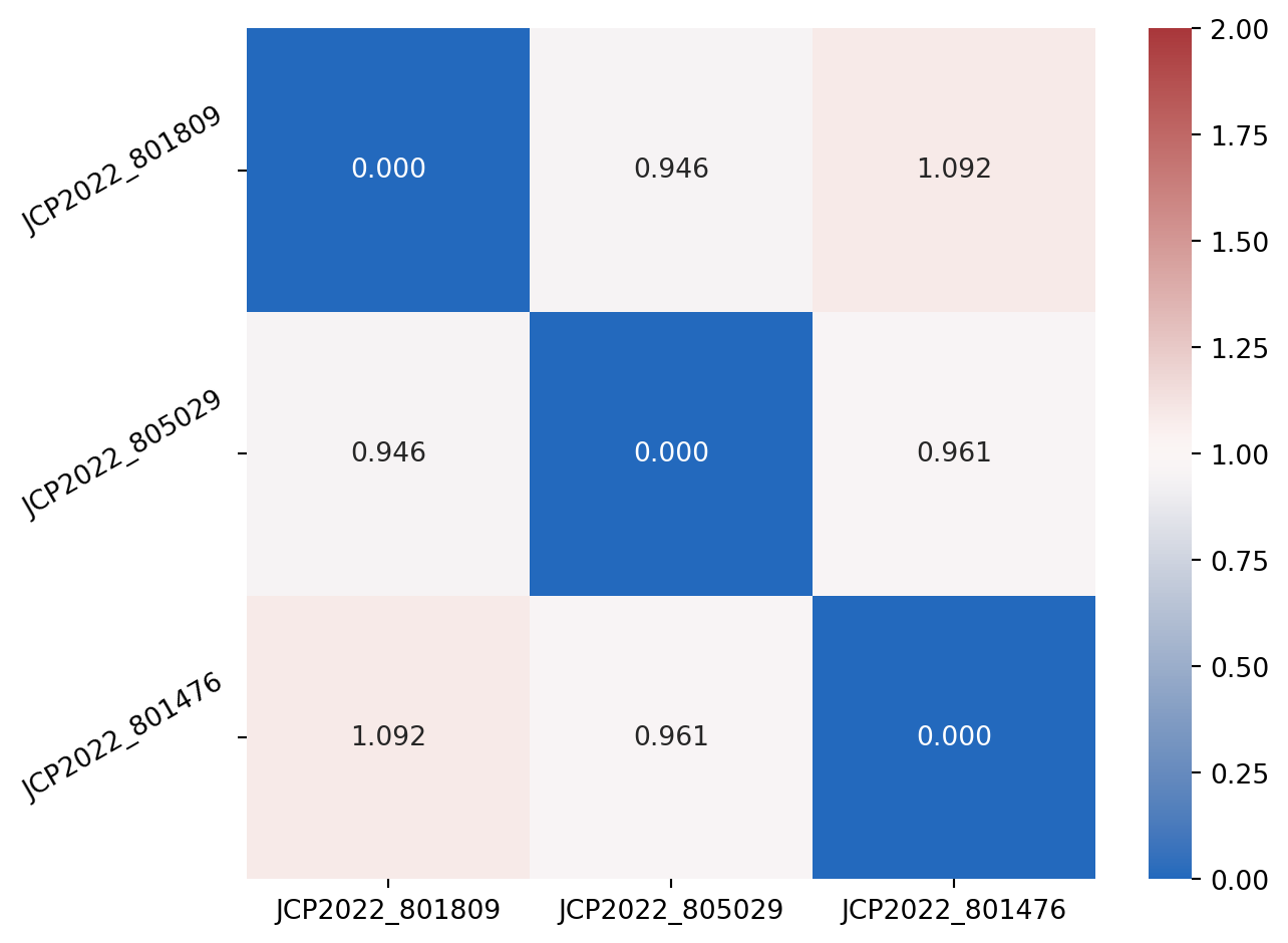

Whilst in this case it is not a terribly interesting result, this shows that we see no correlation between three randomly selected perturbations.

Other Formats