import matplotlib.colors as mpl  # noqa: CPY001
import numpy as np
import polars as pl
from jump_portrait.fetch import get_item_location_info, get_jump_image
from matplotlib import pyplot as plt

#Plot all channels for one site
This notebook demonstrates how to retrieve and plot all channels for one site using the jump_portrait library.
First, we need to get location information telling us where all images corresponding to a specific perturbation can be found. We will use the “get_item_location” function from jump_portrait for this. Here we retrieve image locations for the “RAB30” gene:
gene_info = get_item_location_info("RAB30")
gene_info.shape
Downloading data from 'https://github.com/jump-cellpainting/datasets/raw/c68deb2babc83747e6b14d8a77e5655138a6086a/metadata/well.csv.gz' to file '/home/runner/.cache/pooch/4efbf4dd3dd9aaecc8ccb9fc3c6b4122-well.csv.gz'.
Downloading data from 'https://github.com/jump-cellpainting/datasets/raw/c68deb2babc83747e6b14d8a77e5655138a6086a/metadata/plate.csv.gz' to file '/home/runner/.cache/pooch/a530bb82de29e39332bdef6f29397769-plate.csv.gz'.
worker #0: 0%| | 0/2 [00:00<?, ?it/s]worker #1: 0%| | 0/2 [00:00<?, ?it/s]worker #3: 0%| | 0/2 [00:00<?, ?it/s]worker #2: 0%| | 0/2 [00:00<?, ?it/s]worker #1: 50%|█████ | 1/2 [00:00<00:00, 3.94it/s]worker #3: 50%|█████ | 1/2 [00:00<00:00, 4.65it/s]worker #2: 50%|█████ | 1/2 [00:00<00:00, 2.75it/s]worker #3: 100%|██████████| 2/2 [00:00<00:00, 4.86it/s]worker #3: 100%|██████████| 2/2 [00:00<00:00, 4.83it/s]
worker #4: 0%| | 0/2 [00:00<?, ?it/s]worker #2: 100%|██████████| 2/2 [00:00<00:00, 3.98it/s]worker #2: 100%|██████████| 2/2 [00:00<00:00, 3.73it/s]
worker #0: 50%|█████ | 1/2 [00:00<00:00, 1.67it/s]worker #1: 100%|██████████| 2/2 [00:00<00:00, 2.76it/s]worker #1: 100%|██████████| 2/2 [00:00<00:00, 2.89it/s]
worker #0: 100%|██████████| 2/2 [00:00<00:00, 2.37it/s]worker #0: 100%|██████████| 2/2 [00:00<00:00, 2.23it/s]
worker #4: 50%|█████ | 1/2 [00:00<00:00, 2.06it/s]worker #4: 100%|██████████| 2/2 [00:00<00:00, 2.24it/s]worker #4: 100%|██████████| 2/2 [00:00<00:00, 2.21it/s](90, 47)There are 90 images: 9 sites/well X 5 replicate wells X 2 data types (CRISPR & ORF). We can also retrieve locations for compound data. By default, the function assumes a query by INCHI key. We can also query by JCP ID by specifying the query column:
cmpd_info_byinchi = get_item_location_info("CLETVKMYAXARPO-UHFFFAOYSA-N")
cmpd_info_byjcp = get_item_location_info("JCP2022_011844", input_column="JCP2022")

print(cmpd_info_byinchi.shape)
print(cmpd_info_byjcp.shape)
worker #0: 0%| | 0/1 [00:00<?, ?it/s]worker #1: 0%| | 0/1 [00:00<?, ?it/s]worker #2: 0%| | 0/1 [00:00<?, ?it/s]worker #3: 0%| | 0/1 [00:00<?, ?it/s]worker #3: 100%|██████████| 1/1 [00:00<00:00, 3.65it/s]worker #3: 100%|██████████| 1/1 [00:00<00:00, 3.65it/s]
worker #4: 0%| | 0/1 [00:00<?, ?it/s]worker #1: 100%|██████████| 1/1 [00:00<00:00, 3.05it/s]worker #1: 100%|██████████| 1/1 [00:00<00:00, 3.05it/s]
worker #4: 100%|██████████| 1/1 [00:00<00:00, 5.84it/s]worker #4: 100%|██████████| 1/1 [00:00<00:00, 5.83it/s]
worker #2: 100%|██████████| 1/1 [00:00<00:00, 1.41it/s]worker #2: 100%|██████████| 1/1 [00:00<00:00, 1.41it/s]
worker #0: 100%|██████████| 1/1 [00:00<00:00, 1.34it/s]worker #0: 100%|██████████| 1/1 [00:00<00:00, 1.34it/s]
worker #0: 0%| | 0/1 [00:00<?, ?it/s]worker #1: 0%| | 0/1 [00:00<?, ?it/s]worker #2: 0%| | 0/1 [00:00<?, ?it/s]worker #3: 0%| | 0/1 [00:00<?, ?it/s]worker #2: 100%|██████████| 1/1 [00:00<00:00, 10.90it/s]
worker #4: 0%| | 0/1 [00:00<?, ?it/s](34, 77)
(34, 77)worker #3: 100%|██████████| 1/1 [00:00<00:00, 6.06it/s]worker #3: 100%|██████████| 1/1 [00:00<00:00, 6.05it/s]
worker #1: 100%|██████████| 1/1 [00:00<00:00, 5.05it/s]worker #1: 100%|██████████| 1/1 [00:00<00:00, 5.04it/s]
worker #4: 100%|██████████| 1/1 [00:00<00:00, 7.02it/s]worker #4: 100%|██████████| 1/1 [00:00<00:00, 7.01it/s]
worker #0: 100%|██████████| 1/1 [00:00<00:00, 4.12it/s]worker #0: 100%|██████████| 1/1 [00:00<00:00, 4.12it/s]There are 34 sites corresponding to this compound. We’ve written a function to display all channels for a specific image. Note that this is just one possible way to display images - we’ve included the function here so that you can modify it to suit your own needs.
def display_site(
source: str,
batch: str,
plate: str,
well: str,
site: int,
label: str,
int_percentile: float,
) -> None:
"""Plot all channels from one image.
Parameters
----------
source : String
Source ID for image of interest.
batch : String
Batch ID for image of interest.
plate : String
Plate ID for image of interest.
well : String
Well ID for image of interest.
site : String
Site ID for image of interest.
label : String
Label to display in lower left corner.
int_percentile: float
Rescale the image from 0 - this percentile of intensity values.
"""
n_rows = 2
n_cols = 3
# Make images
axes = plt.subplots(n_rows, n_cols, figsize=(2.6 * n_cols, 2.6 * n_rows))[1]
axes = axes.ravel()
channel_rgb = {
"AGP": "#FF7F00", # Orange
"DNA": "#0000FF", # Blue
"ER": "#00FF00", # Green
"Mito": "#FF0000", # Red
"RNA": "#FFFF00", # Yellow
}
for ax, (channel, rgb) in zip(axes, channel_rgb.items()):
cmap = mpl.LinearSegmentedColormap.from_list(channel, ("#000", rgb))
img = get_jump_image(source, batch, plate, well, channel, site, None)
ax.imshow(img, vmin=0, vmax=np.percentile(img, int_percentile), cmap=cmap)
ax.axis("off")
# Add channel name label in the top left corner
ax.text(
0.05,
0.95,
channel,
horizontalalignment="left",
verticalalignment="top",
fontsize=18,
color="black",
bbox=dict(
facecolor="white", alpha=0.8, edgecolor="none", boxstyle="round,pad=0.3"
),
transform=ax.transAxes,
)
# put label in last subplot
ax = axes[-1]
ax.text(
0.5,
0.5,
label,
horizontalalignment="center",
verticalalignment="center",
fontsize=20,
color="black",
transform=ax.transAxes,
)
ax.axis("off")
# show plot
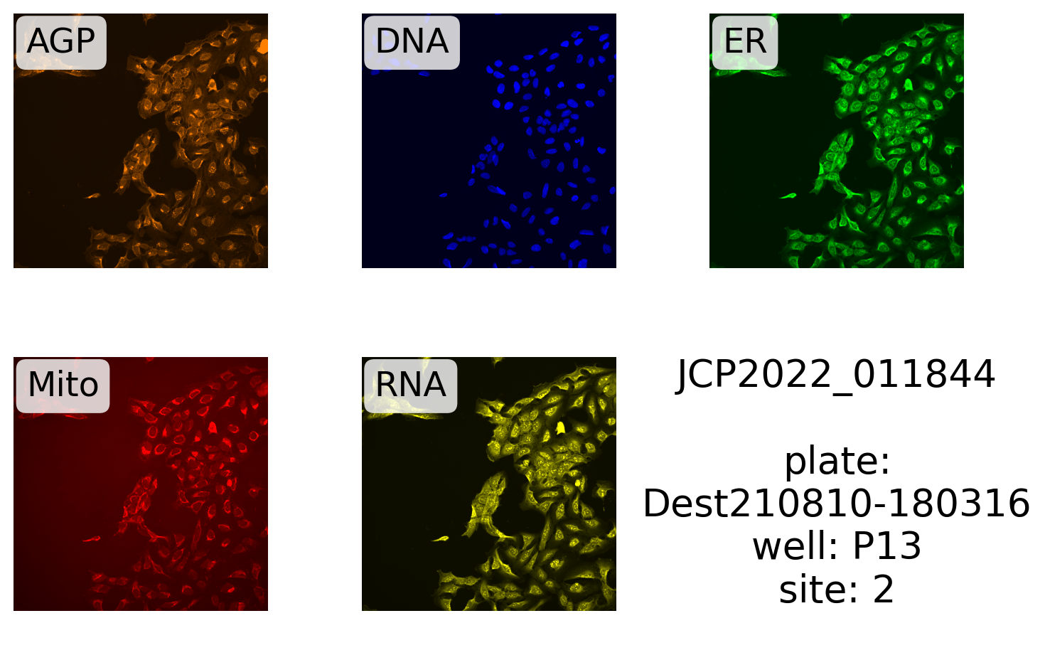
plt.tight_layout()We can get the required location parameters from the location info that we retrieved earlier. Here we get parameters for the first site in the JCP compound results:
(
    source,
    batch,
    plate,
    well,
    site,
) = cmpd_info_byjcp.select(
    pl.col(f"Metadata_{x}" for x in ("Source", "Batch", "Plate", "Well", "Site"))
).row(0)
Next, we define the label and make the plot:
label = "{}\n\nplate:\n{}\nwell: {}\nsite: {}"

display_site(
    source,
    batch,
    plate,
    well,
    site,
    label.format("JCP2022_011844", plate, well, site),
    99.5,
)
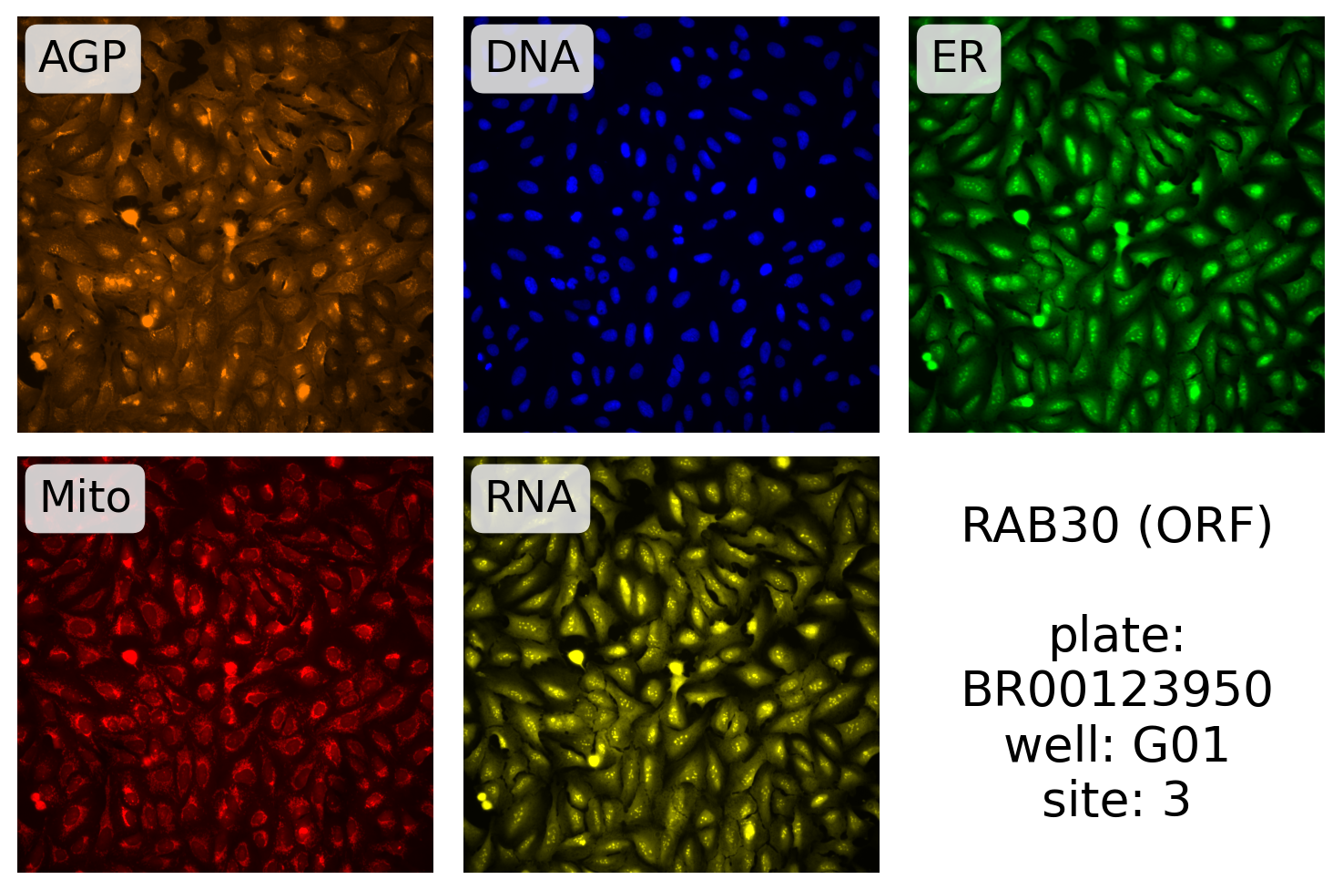
Here, we plot one of the RAB30 ORF images:
source, batch, plate, well, site = (
    gene_info.filter(pl.col("Metadata_PlateType") == "ORF")
    .select(
        pl.col(f"Metadata_{x}" for x in ("Source", "Batch", "Plate", "Well", "Site"))
    )
    .row(0)
)
display_site(
    source,
    batch,
    plate,
    well,
    site,
    label.format("RAB30 (ORF)", plate, well, site),
    99.5,
)
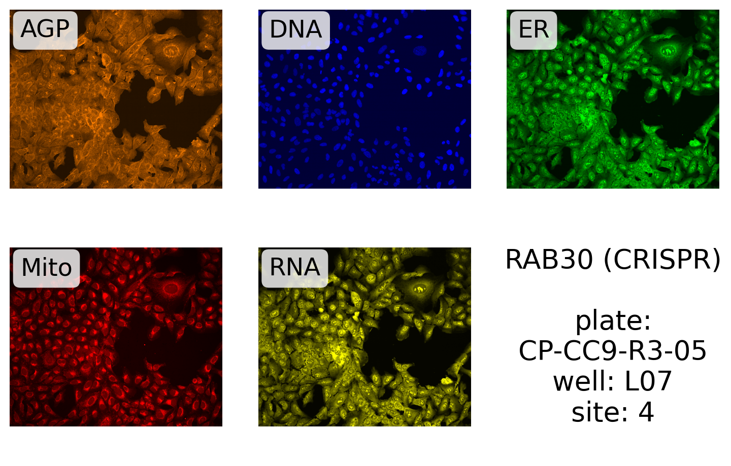
And for CRISPR:
source, batch, plate, well, site = (
    gene_info.filter(pl.col("Metadata_PlateType") == "CRISPR")
    .select(
        pl.col(f"Metadata_{x}" for x in ("Source", "Batch", "Plate", "Well", "Site"))
    )
    .row(0)
)
display_site(
    source,
    batch,
    plate,
    well,
    site,
    label.format("RAB30 (CRISPR)", plate, well, site),
    99.5,
)