Day 3, Exercise 1: Practical introduction to ilastik

Day 3, Exercise 1: Practical introduction to ilastik#

Lab authors: Kyle Karhohs, Mario Cruz, Beth Cimini .

Learning Objectives#

Learn how ilastik can easily create probability maps that look like fluorescence
Export data from ilastik to use it in a downstream program (in this case, CellProfiler)
Try ilastik in 3D, and examine the effect of your noise on your probability predictions

Lab Data in for Exercise 1 available here, for Exercise 2 available here

Introducing Ilastik#

Despite the many problems CellProfiler can readily solve, certain types of images are particularly challenging. For instance, when the biologically relevant objects are defined more by texture and context than raw intensity many classical image processing techniques can be foiled; DIC images of cells are a common biological example.

Thankfully, machine learning, particularly [pixel-based classification] has yielded powerful techniques that can often solve these challenging cases. ilastik is an open-source tool built for pixel-based classification, and, when combined with CellProfiler, the range of biology that can be quantified from images is greatly expanded beyond monocultures of monolayers to include increased complexity such as tissues, organoids, or co-cultures.

Now, let’s take a look at how ilastik can be used together with CellProfiler!

Exercise 1: Using ilastik to turn 2D phase images into pseudo-fluorescence#

Step 1: The DIC conundrum#

Consider segmenting DIC images, such as those within the imageset BBBC030. The goal will be to identify individual Chinese Hamster Ovary (CHO) cells and the regions they occupy.

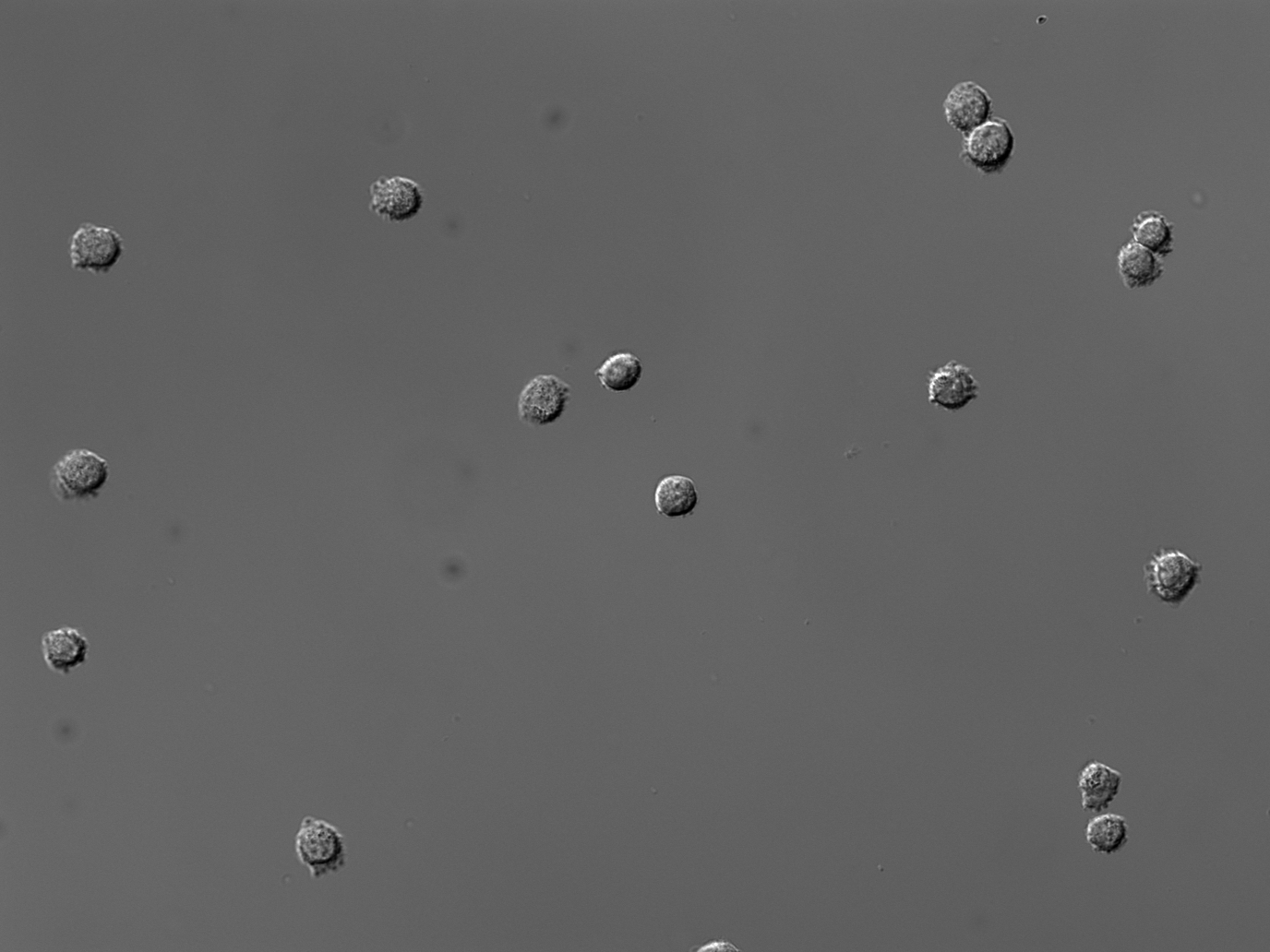
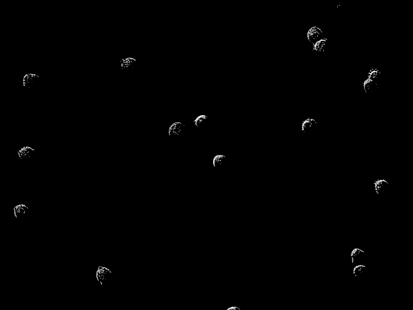
A straightforward thresholding of this image yields poor results, because the cells have almost the same pixel intensity values (and sometimes even darker!) as the background. There is therefore no true foreground for these cells based solely upon an intensity histogram. Thresholding renders the CHO cells into moon-like crescents. While these fragments could be useful for simple cell counting, most metrics of morphology will be inaccurate. Now, note that there is a module, EnhanceOrSuppressFeatures, that is specifically capable of transforming DIC images into something that is readily segmented. But let’s pretend for a moment we didn’t have that option…

Step 2: Pixel-based classification with Ilastik#

ilastik employs pixel-based classification and complements CellProfiler. The CHO cells within the DIC image are obvious to the human eye, because we can discern that each cell is defined by a characteristic combination of light and dark patterns. These same patterns can be detected with the machine-learning algorithms within ilastik.

The machine-learning implemented by ilastik requires user annotation about what is background and what is a CHO cell before it can automatically make this determination across a set of images. ilastik provides a user interface for labeling, tagging, and identifying the objects of interest within an image. This annotation creates what is referred to in machine learning as a training set.

Annotation with 2 Labels#

Open ilastik
Start a Pixel Classification project.
Load at least several BBBC030 images by drag-and-drop into the Input Data window.

Now explore the image within the ilastik gui. Here are some shortcuts that may prove useful are:
- Ctrl + mouse-wheel = zoom.
- The keyboard shortcut Ctrl-D will show the grid Ilastik uses to partition the image for processing.
- Zoom-in far enough that the grid is no longer visible. This will speed up the Live Update.
Open the Feature Selection window and add all features.
Open the Training window.
Rename the two label classes (if you like, so you don’t get confused) to something like Cells and Background
Using the paint brush tool, label pixels (one at a time) for each class until you are satisfied with the segmentation.

Tip

Accidentally made the background class first? No problem, you can either clear the labels and start over, or we can show you how to change CellProfiler’s expectations for the channel order later

We recommend creating labels for each class one pixel at a time, rather than by making scribbles, to minimize the chance of [over-fitting], i.e. too much information about any given area can cause classification to do poorly in other slightly-dissimilar areas. To label one pixel at a time, we’ll need to zoom in far enough to resolve the individual pixels in the image. The image below shows how closely we must view individual cells before the pixels of the image become clear.

Using a brush size of 1, we click a single pixel from each class: one within a single CHO cell and the other in the surrounding background. In the next image, the annotation color of the CHO cell is yellow and the annotation color of the background is green. Activating Live Update reveals the segmentation looks similar to the results from thresholding. This outcome is promising considering this classification was determined by 1 feature and 1 pixel each for the CHO and background labels.

Adding more labels, one pixel at a time, we continue to refine the segmentation. Toggling the Segmentation and Uncertainty views provides real-time feedback that can guide the labeling process. Areas of high uncertainty will be aqua-blue, so annotating those areas will be most beneficial to training the program which pixels belong to which class. You should also view the predicted segmentation, and annotate pixels that are not currently segmented properly.

Continue until it seems that additional labels do not change the results, or a subset of the pixels begin “flipping” between CHO cell and background, or until you’ve labeled ~20 pixels in your original region. Check and label other cells in the image, as well as in other images, to make sure the diversity in your experiment is represented in the training set.

Export the probability maps#

When satisfied with the results, export the probability maps.

Open the Prediction Export window.
Click the Choose Export Settings window.
Change Transpose to Axis Order to cyx.
Change Format to tiff.
Change the Convert to Datatype to integer 16 bit
Check the button next to Renormalize [min,max]. After all these setting changes, your settings should look like below

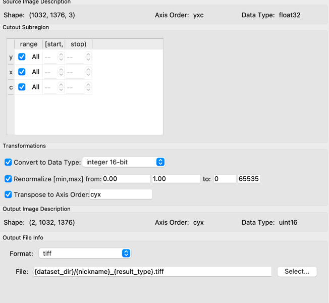
Close the export settings dialog box and click the Export All button.
If you did not initially load all the images into ilastik and wish to create predictions for them all now, go to the Batch Processing window, select the remaining unpredicted images and hit Process all files. This will take a couple of minutes on most computers.
Note that you’re producing a two channel image (Color Image).

Step 3: Segmenting probabilities with CellProfiler#

The probability map images created with ilastik can then be processed by CellProfiler to identify and measure the CHO objects within the DIC images. The probability map images are grayscale images and can be treated as if they were the result of a “stain” for the cells.

Open CellProfiler.
Load the pixel_based_classification.cpppipe pipeline file.
Add the exported probability images AND their matching original images to the Images module.

Tip

If you HAVE run all of the images through ilastik, you can just drag and drop the whole folder in. If you haven’t, you should drag and drop in only the pairs of .tiffs and .pngs that you have run - or CellProfiler will get confused how to match them (without doing extra work in the NamesAndTypes module)

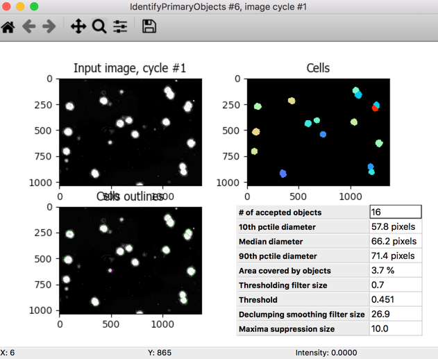
Enter test mode, run the pipeline, and see what happens!

You should see something like the image below in your IdentifyPrimaryObjects module - thanks to ilastik, we have now transformed the patterns and texture of intensity in the DIC image into an image where the intensity reflects the likelihood that a given pixel belongs to a cell. The image below demonstrates how the IdentifyPrimaryObjects module successfully segments all the CHO cells.

(Optional) Didn’t get that? Is it possible that in ilastik, your first class was your background and your second class was the cells? No problem! In the ColortoGray module, simply switch from splitting out the Red channel to the Green channel, and be sure to change the name of the split out Green channel to what the Red channel had been (choSegmented) before turning the Red channel segmentation off.
(Optional): examine the NamesAndTypes module; do you understand why everything is set the way that it is?
(Optional): the first Threshold module isn’t being used in your pipeline, it’s just a demonstration to show you how poorly threshold would perform on the raw images. Is it better or worse than you expected?
Exit test mode, set your Default Output Folder to something reasonable, and run the pipeline and review the segmentation images saved to disk. How robustly did it perform on different images?

Exercise 2: Using ilastik on 3D simulated data#

We discussed earlier overfitting -let’s see if we can make it happen in action, while trying out some of ilastik’s 3D capabilities!

Our dataset here comes from the Association of Biomolecular Research Facilities - Light Microscopy Research Group (ABRF/LMRG); they made synthetic images of FISH staining in C. elegans which vary in their signal-to-noise ratio and the clustering of their objects. Their goal was for people to submit workflows in different tools, so they could assess the accuracy of the workflows people created.

Images 1 and 2 have low noise, while images 3 and 4 have high noise; images 1 and 3 have FISH spots that are not very clustered, whereas 2 and 4 have lots of spot clusters.

Initiating the project#

Start a new pixel classification project in ilastik
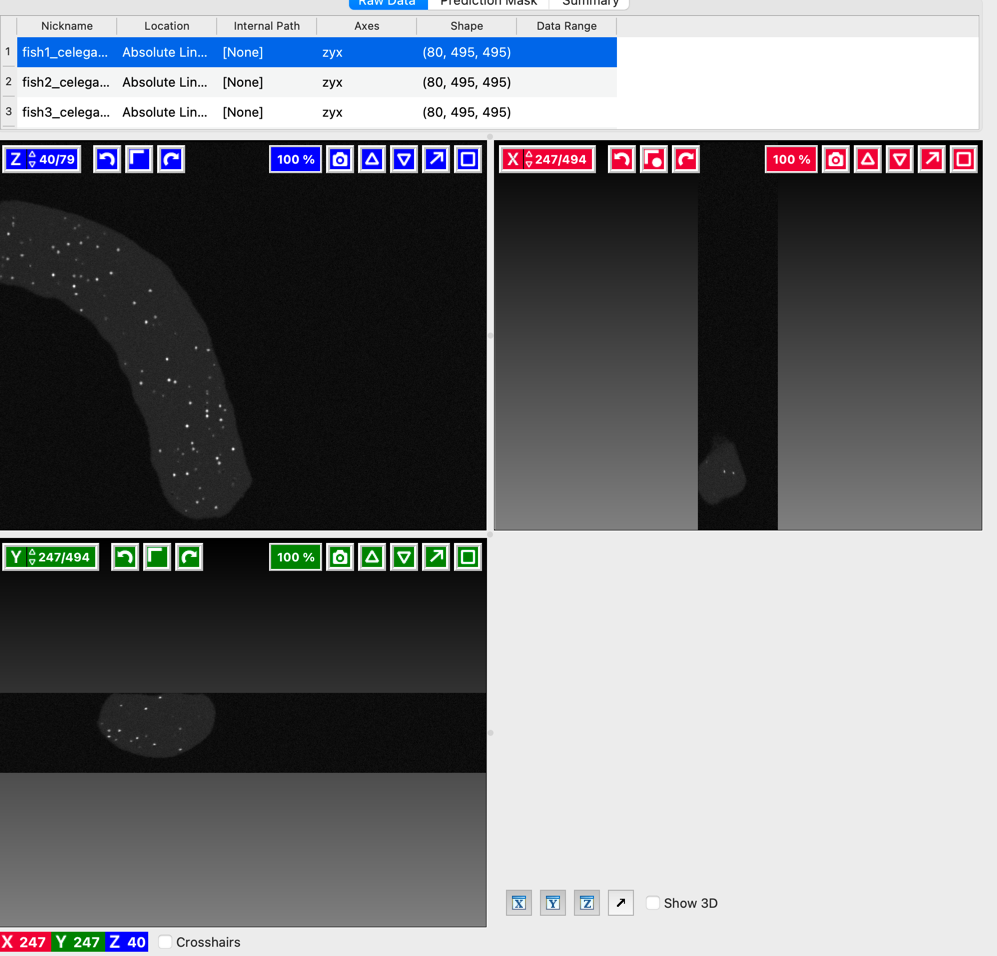
Drag the new images in
Examine ilastik’s 3D viewer - you can look at the images in XY, XZ, and YZ. Can you imagine a time that would be helpful?

Enable all of the features

Labeling the first image#

Add a third class of label, and then rename your labels - in any order, you should have a class for background, a class for the body of the worm, and a class for the actual FISH spots themselves
On the first image (and only the first image), annotate just a few pixels in each class
Turn on live update - how does it look? If not great, annotate just a couple of other pixels until the prediction looks decent.

Look at the other images#

Switch to image 2 - how does it look compared to image 1?
Switch to images 3 and 4 - how does it compare to image 2, which also hasn’t been annotated but has a similar noise distribution?

Look at the effect of feature size on prediction time, accuracy, and generalization#

Return to image 1, and turn off Live Update
Click Suggest Features
This menu is designed to help you pick out a subset of features from a single image’s annotations that work the best (where best for you might be “fastest” or “best performing” - it will show you both) - this can be especially important for 3D where in large images feature calculation can be very slow.

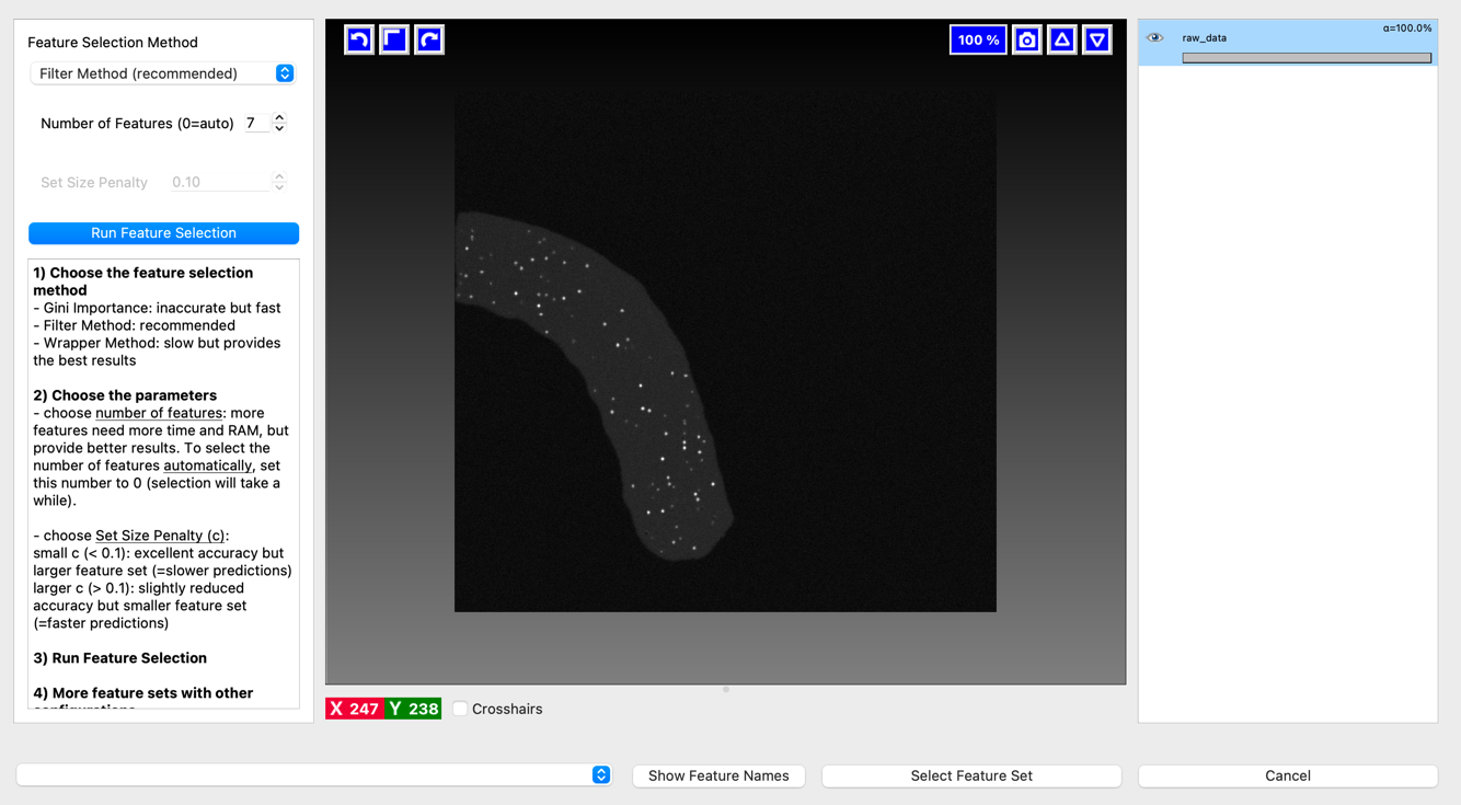
Hit Run Feature Selection to have ilastik pick out a set of 7 (or other, if you change the number) features it thinks will do the best job on this image. This may take a minute or two.
Look at the bottom left of the menu - it will show you performance on your features in terms of time taken and accuracy on this image. How do these compare between 7 features and all features?
(Optional) Hit Show Feature Names
Select ilastik’s recommended 7 features and pick Select Feature Set to pick them.

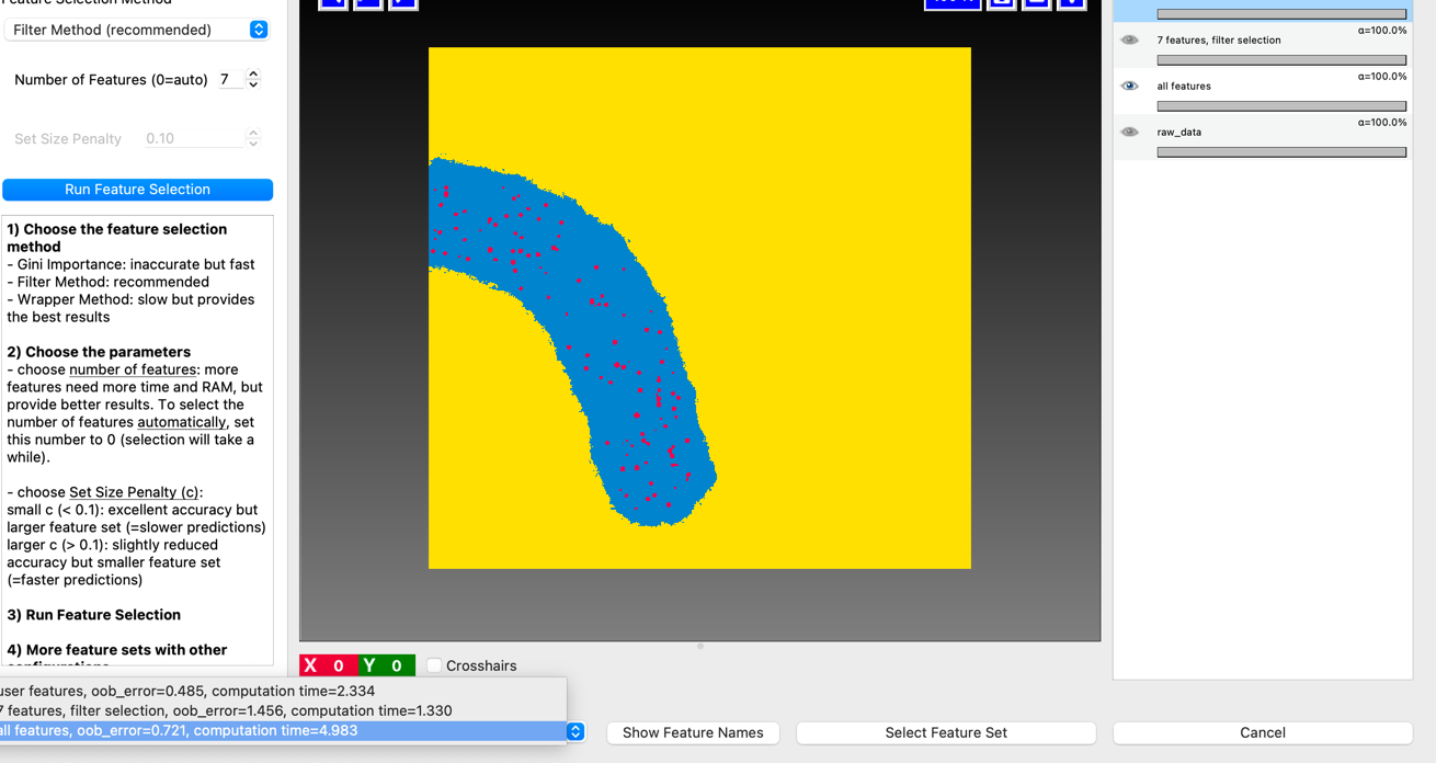
Turn live update back on and check generalization to other images again - is it better or worse than with all the features?
(Optional) - turn live update back off, return to the feature selection menu, and rationally pick a subset of the features - maybe one or two sigma values, and/or one or two categories. Return to the training menu, pull up image 1, and then go back to the Select Features menu - how does your rational set of features compare in accuracy and time to all the features or the optimal 7? How about in generalization, if you select them?