Day 3, Exercise 2: Practical introduction to QuPath

Lab author: Shatavisha Dasgupta .

Adapted from:

1. QuPath documentation

2. Pete Bankhead’s video tutorial

3. From Samples to Knowledge 2025 Repo

Learning Objectives

This tutorial provides an overview of the basic functionalities of QuPath. Specifically, the tutorial covers the following:

• Creating a QuPath project

• Viewing pyramidal files

• Setting channel names of images

• Manually annotating regions of interest

• Detecting cells in the annotated regions

• Performing measurements on the detected cells and exporting the data

Lab Data in this folder (Originally sourced from here and here)

━━━━━━━━━━━━━━━━━━━━━━━━━━━━━━━━━━━━━━━━━━━━━━━━━━━━━━━━━━━━━━━━

1. Background information

1.1 What is QuPath?

---

QuPath is an open source software for bioimage analysis created and maintained by Peter Bankhead and his team at The University of Edinburgh. QuPath is commonly used for digital pathology in research because it offers a powerful set of tools for working with whole slide images - but it can be applied to lots of other kinds of image as well.

Read the original publication introducing QuPath!

QuPath provides powerful tools for annotation, visualization, and image analysis through an easy-to-use modern interface. It includes built-in algorithms for cell and tissue detection, interactive machine learning for object and pixel classification, and supports many image formats, including whole-slide and multiplexed images. It also integrates with tools like ImageJ, OpenCV, OMERO, StarDist, InstanSeg, and Bio-Formats, and the functionalities can be expanded using Groovy scripts and extensions. Many of these functionalities are beyond the scope of this tutorial – if you are interested, QuPath docs and these videos/channels (1, 2, 3) are great resources to delve into!

1.2 What are pyramidal file formats?

---

• Whole slide images (WSIs) are a crucial component of translational research focussing on Histopathology, because they allow comparing changes in diseased tissue with healthy tissue, which are often present on the same slide. Additionally, they also allow quantifying parameters of prognostic significance, such as depth of invasion of tumors

• WSIs contain a wealth of information – and billions of pixels – so these tend to be of substantial size, often exceeding 10 GB

• To make viewing, processing, and analysis more efficient, WSIs are commonly stored in pyramidal file formats

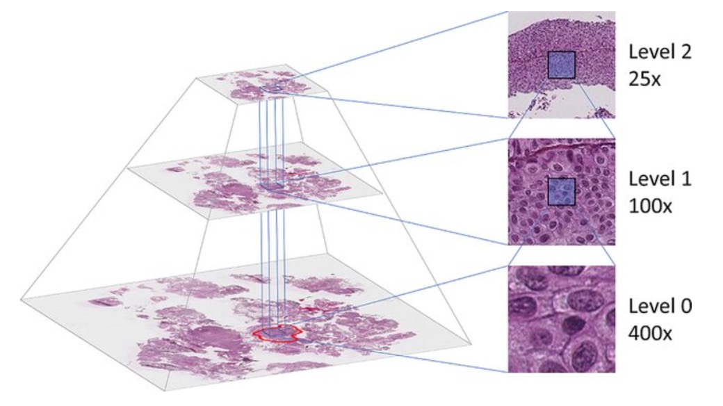
• A pyramidal file stores the same image at multiple resolutions within a single file. These resolutions are arranged in a pyramid-like hierarchy, with the full-resolution image at the base and progressively lower-resolution versions above it

• This allows the software to load only the resolution needed for a given zoom level, rather than loading the entire high-resolution image into memory

• In histology, this is especially useful because low-resolution views allow rapid navigation across the tissue, while high-resolution views allow detailed examination of cellular and tissue structures

• As shown in the figure, pyramidal images are typically organized as:

  • Level 0: Full-resolution image

  • Higher levels: Downsampled versions, such as 1/2, 1/4, or 1/8 scale

• Common use cases include:

  • Digital pathology: .svs, .scn, .ndpi, .tiff

  • Spatial biology: .tiff, .ome.tiff

  • Geospatial imaging: GeoTIFF

• Pyramidal file formats offer several advantages for large-image analysis:

  • Faster loading and rendering

  • Lower memory usage during visualization

  • Efficient low-resolution previews

  • Region-of-interest extraction without decoding the entire image

• Limitations:

  • Pyramidal files can be larger because they store multiple resolutions

  • They often require specialized software for reading, writing, or processing

• Common File Formats:

  • TIFF-based formats such as .tiff and .ome.tiff

  • Vendor-specific formats such as .svs (Aperio), .ndpi (Hamamatsu), or .scn (Leica)

• These files can be read using tools such as:

  • OpenSlide

  • Bio-Formats

  • pyvips

  • tifffile

  • QuPath

━━━━━━━━━━━━━━━━━━━━━━━━━━━━━━━━━━━━━━━

2. Exercise steps

2.1 PART I

• 2.1.1 Install and launch QuPath

• 2.1.2 Create a QuPath project

• 2.1.3 Add or remove images to your QuPath project

• 2.1.4 View and export images

• 2.1.5 Set up image properties

• 2.1.6 Annotate images

• 2.1.7 View and export annotation measurements

2.2 PART II

• 2.2.1 Create a QuPath project

• 2.2.2 Annotate the region of interest

• 2.2.3 Perform positive cell detection

• 2.2.4 Annotate areas within the region of interest

• 2.2.5 Create and run object classifier

• 2.2.6 View and export detection measurements

━━━━━━━━━━━━━━━━━━━━━━━━━━━━━━━━━━━━━━━

2.1 PART I

2.1.1 Install and launch QuPath

---

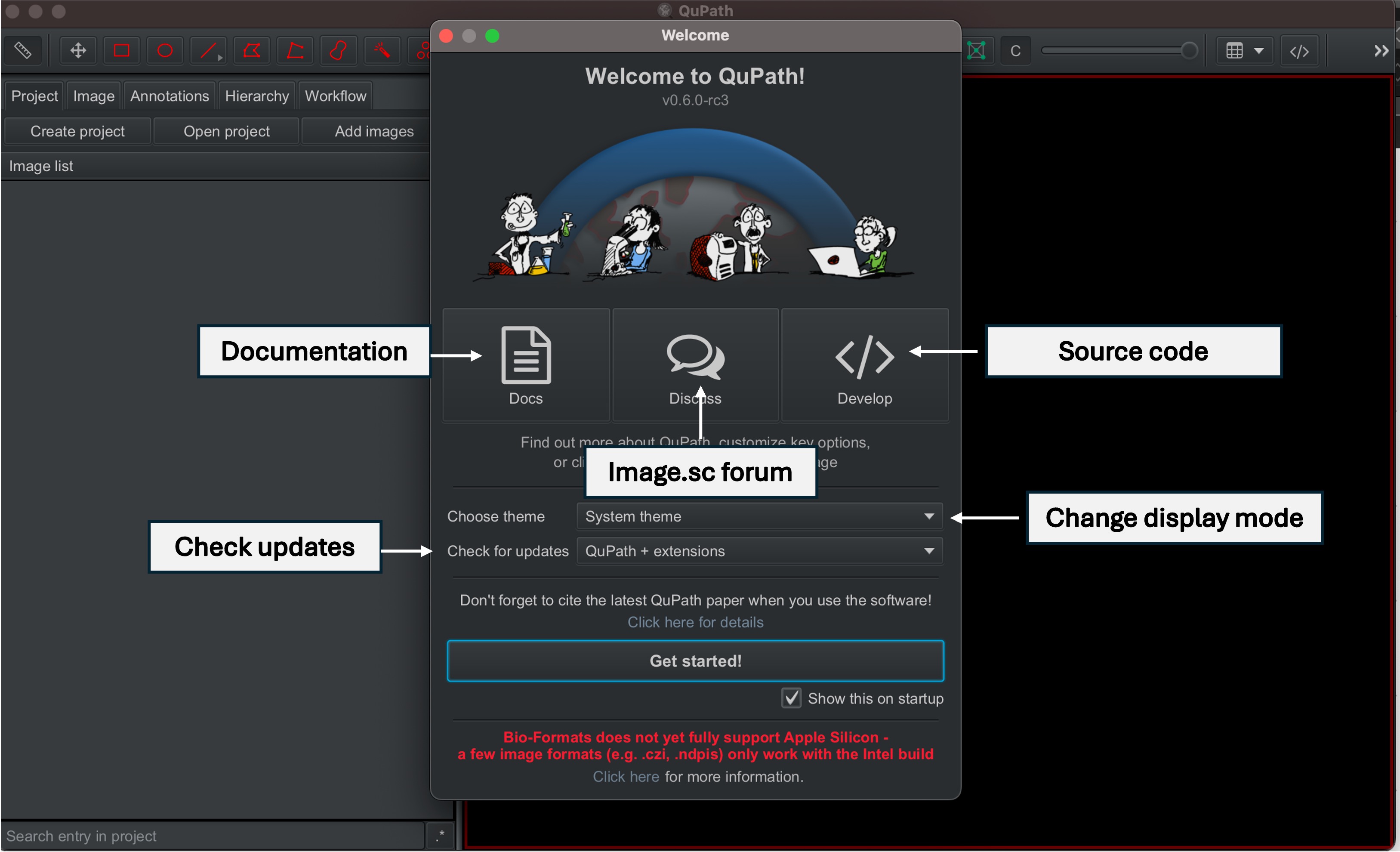
Please install the latest version from here Once installed, click on the QuPath icon, and wait for QuPath to launch. When the QuPath window opens, you will notice the welcome screen, which links to QuPath documentation, the image analysis forum, and also the source code

2.1.2 Create a QuPath project

---

Although it is possible to view and work with single images in QuPath, creating a “Project” makes saving and reloading data associated with multiple images much more efficient. A QuPath project groups related images to easily switch between them via thumbnails and also organizes associated data files, scripts, and classifiers.

We start by creating a “project folder”, which can be any folder, stored anywhere on your computer, but it must be empty.

This can be done by doing either of the following:

1. Click on File; then Project and Create project

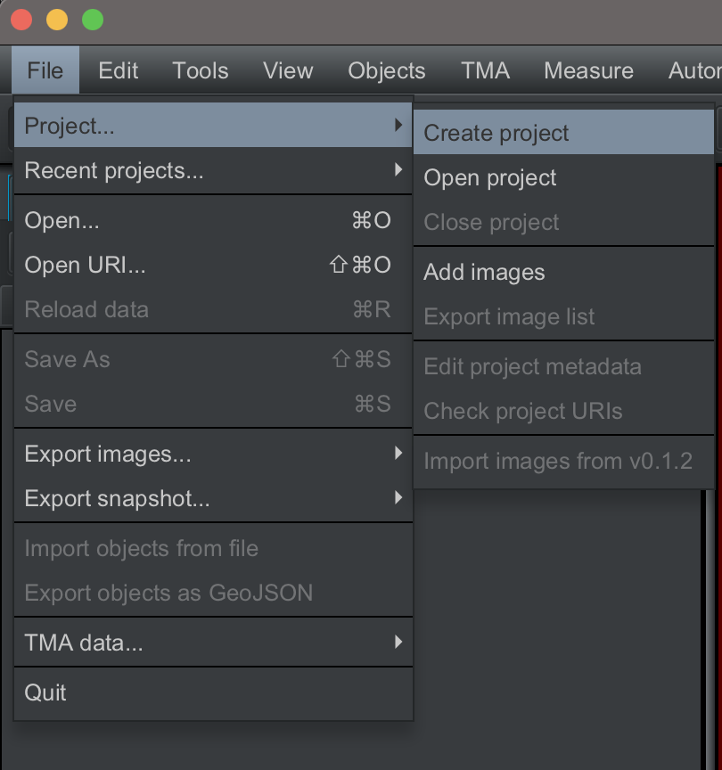
2. Clicking on the Create project button in the analysis pane

3. Dragging and dropping the project folder into QuPath

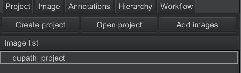
You can name the project anything you like – for this tutorial, I have named it qupath_project. Once the project is created, the project name will appear in the analysis pane.

2.1.3 Add or remove images to your QuPath project

---

2.1.3.1 Add images

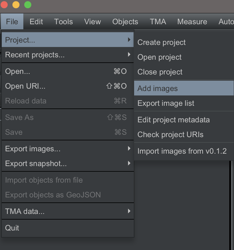
You can add images via File --> Project --> Add images. If you have not created a project and just want to open an image, you can also click on File --> Open. Alternatively, you can drag and drop your images into QuPath – this might be the more efficient option if you are working with a multiple images.

Let us start by importing the image CMU-1.ndpi. This is a hematoxylin-eosin stained section of skin scanned by Hamamatsu scanner.

When you import the image, a dialog box will open where you can set parameters related to the image being imported, as shown below.

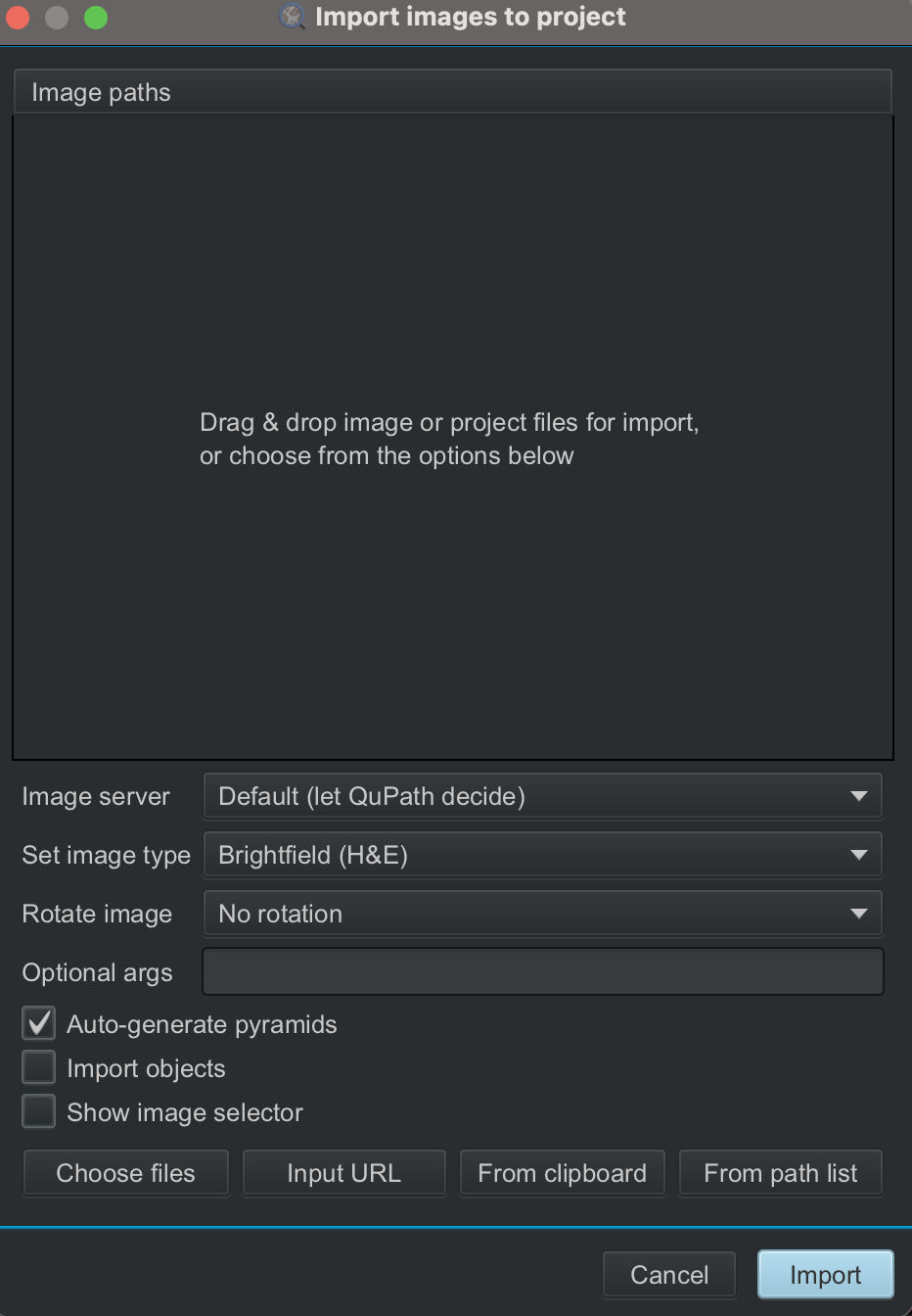
The image CMU-1.ndpi is a brightfield, H&E image, so we set the image type accordingly, and leave all other parameters unchanged, because we do not want to rotate the image right now, and there are no objects to import along with the image.

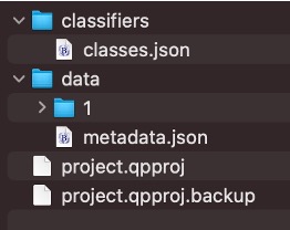
Once the image(s) have been added to your project, you will see some folders created in your project folder.

qupath_project
├── classifiers
│   └── classes.json
├── data
│   ├── 1
│   │   ├── data.qpdata
│   │   ├── server.json
│   │   ├── summary.json
│   │   └── thumbnail.jpg
│   └── metadata.json
├── project.qpproj
└── project.qpproj.backup

2.1.3.2 Remove images

To remove an image, right-click on the image thumbnail in the analysis pane, and select Remove image.

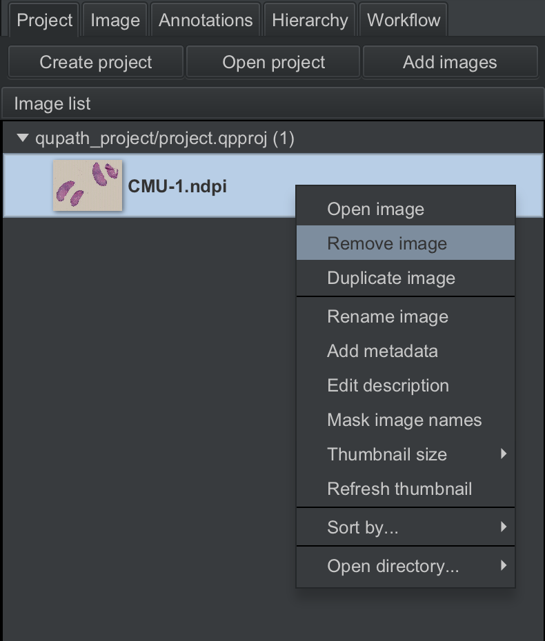
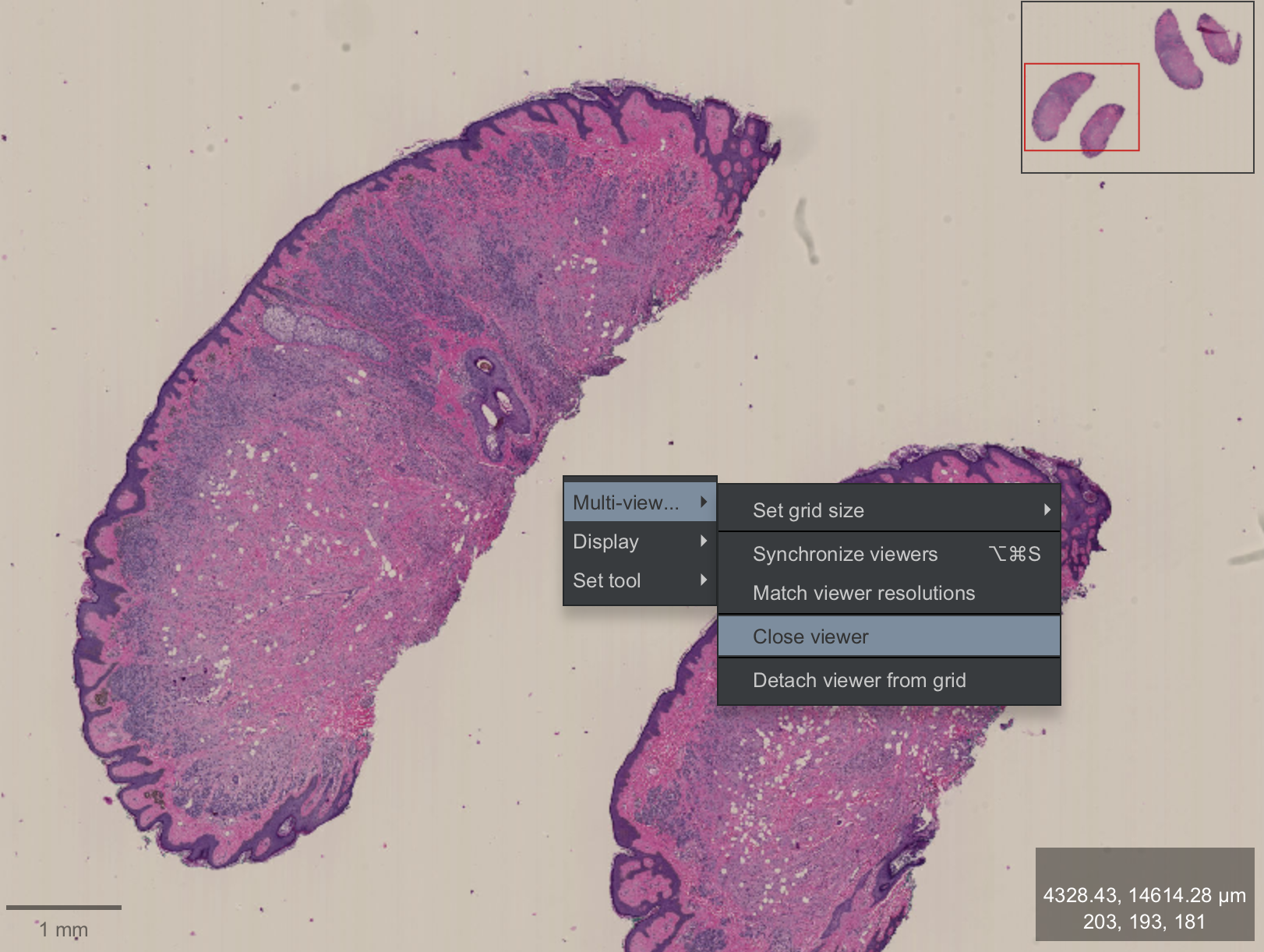
⚠️ Tip: If your project has only once image, or if you have added only one image to your project and want to remove it, make sure to close the viewer by right-clicking anywhere in the viewer, and clicking on Multi-view.. --> Close viewer.

⚠️ Tip: QuPath projects usually do not contain the images, but saves the path where your images are located. If you change the location of the images since creating the project, QuPath may have trouble finding the images when you re-open your project. QuPath does try to help by providing a dialogue box highlighting the paths that are missing and providing some suggestions of file paths where it thinks the images might be located. This dialogue box will also have a Search… button, with which you can set the new directory where the images are now located. Clicking on Apply changes will update the project with the new file paths!

2.1.4 View and export images

---

2.1.4.1 Customize the viewer

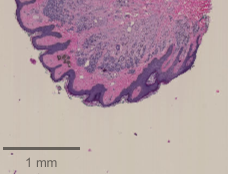
Once you have imported the image(s) to your project, you will see the name(s) of these image(s) in the analysis pane (red box), and the image in the image viewer.

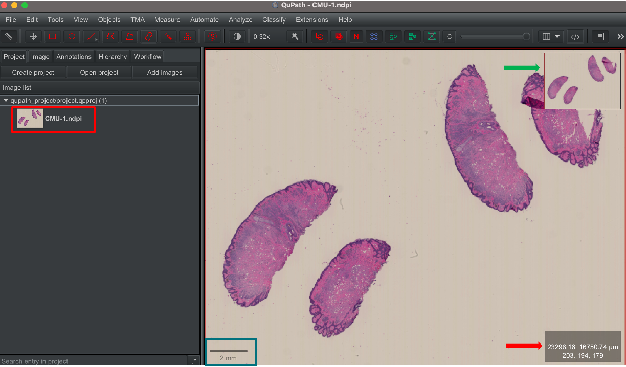
In the viewer pane, you will notice the following:

1. Slide overview (green arrow)

2. X and Y co-ordinates and pixel values for the channels in the image (red arrow)

3. Scale bar (green box)

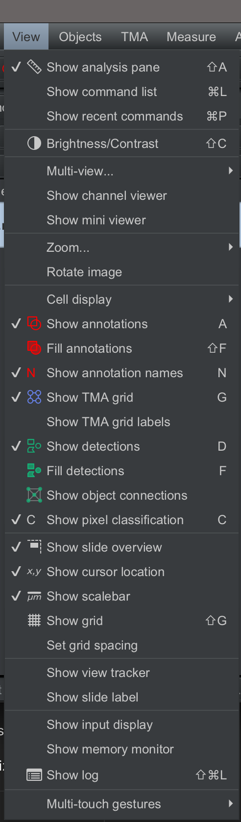
This is a good time to familiarize yourself with the options available under the View button. You will notice that there are options to toggle on or off the slide overview, analysis pane, scale bar and so on.

2.1.4.2 Zooming and panning

The scroll wheel of your mouse (or equivalent scrolling motion on a trackpad) can be used to zoom in and out of an image within QuPath.

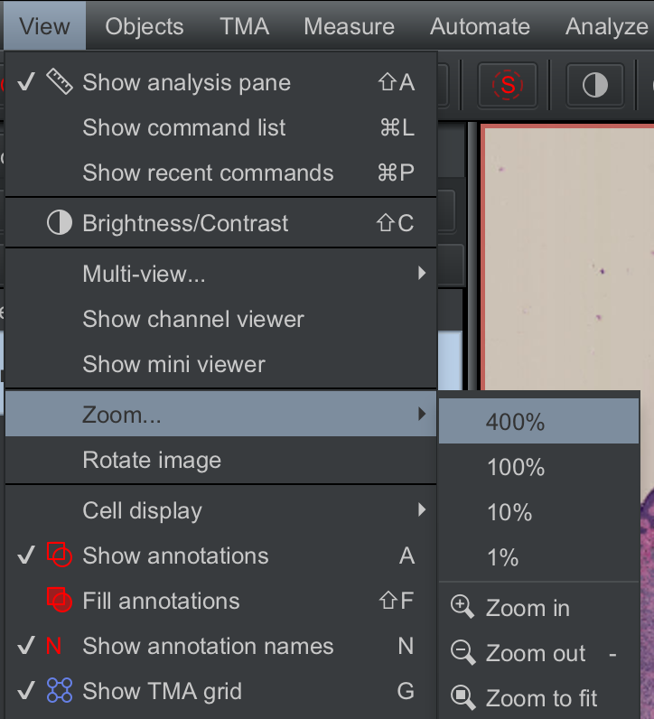
Alternatively, you can click on View and Zoom to zoom in or out, or to zoom to specific magnifications (e.g. 400%)

⚠️ Tip: You can also navigate to a specific part of the WSI by clicking on that area in the slide overview window.

You can pan the image with the move tool (red box) and clicking on the magnifying glass icon (green box) will fit the image to the viewer.

2.1.4.3 Export images

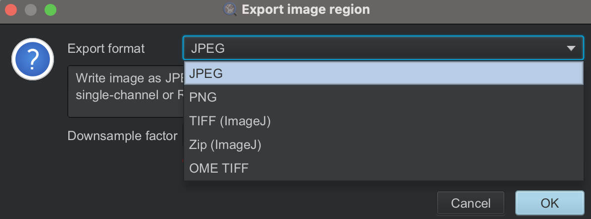
QuPath can also be handy for preparing figures for your publications or presentations. The Export images button under File provides several options for exporting an image.

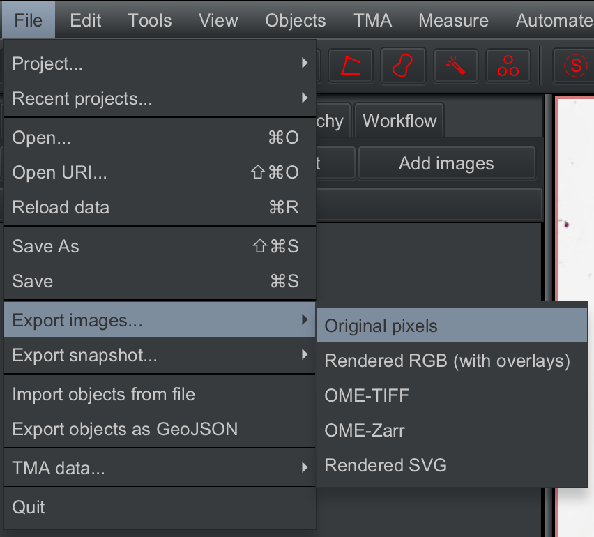
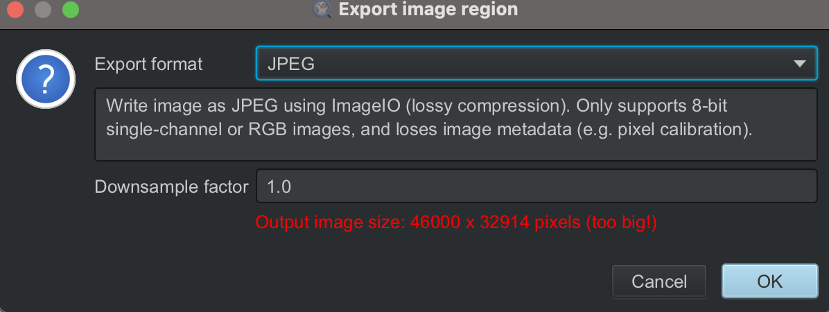
If you select Original pixels, you will be provided a list of available file formats for saving the image.

Selecting Rendered RGB (with overlays) exports the image as it appears in the QuPath viewer, including overlays. Please remember that because the image is converted to RGB, the exported pixel values may not match the original data. This option is therefore suitable for preparing figures, but not for downstream quantitative analysis.

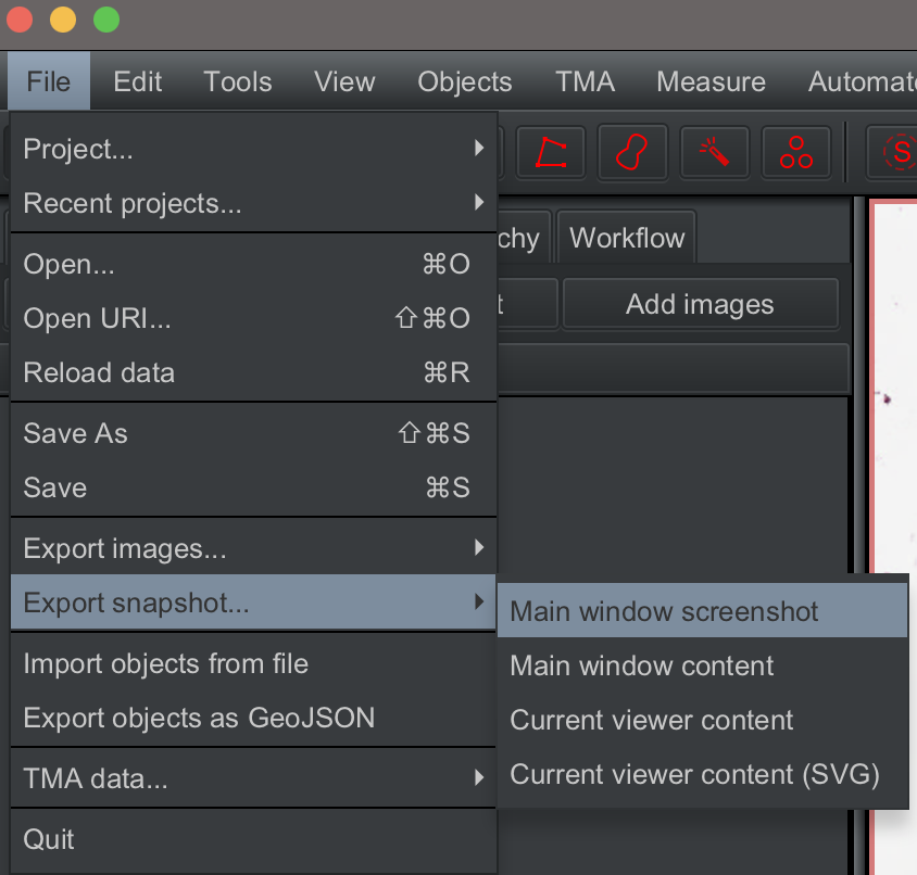
The Export snapshot button includes two additional options that allow more of the QuPath interface to be exported, such as toolbars and panels.

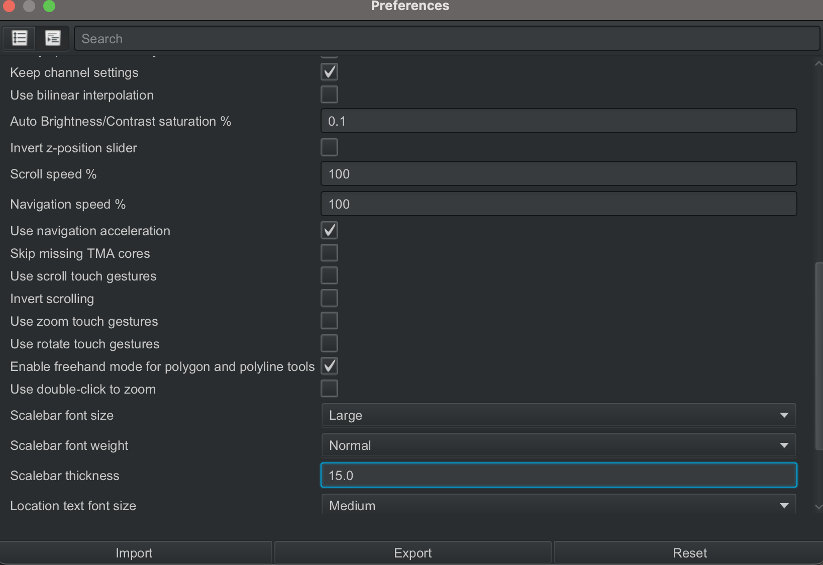
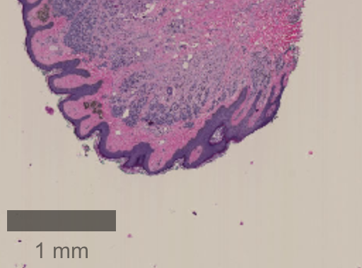
⚠️ Tip: You can change the appearance of the scalebar by clicking Edit --> Preferences and changing the parameters for Scalebar under the Viewer tab. The screenshot below shows the default parameters and appearance of the scalebar when default parameters are used.

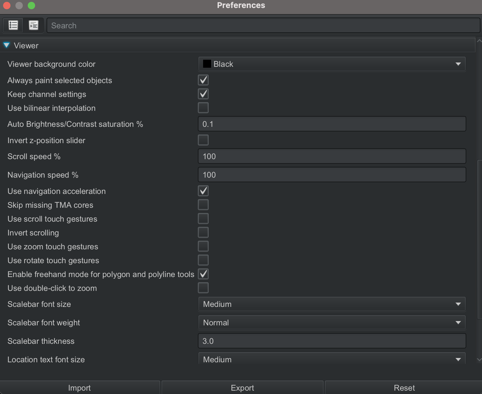
You can always change the Scalebar font size, font weight and thickness according to your preference, as shown below, and the changes will be reflected in the scalebar in the viewer.

2.1.5 Set up image properties

---

2.1.5.1 Set image type

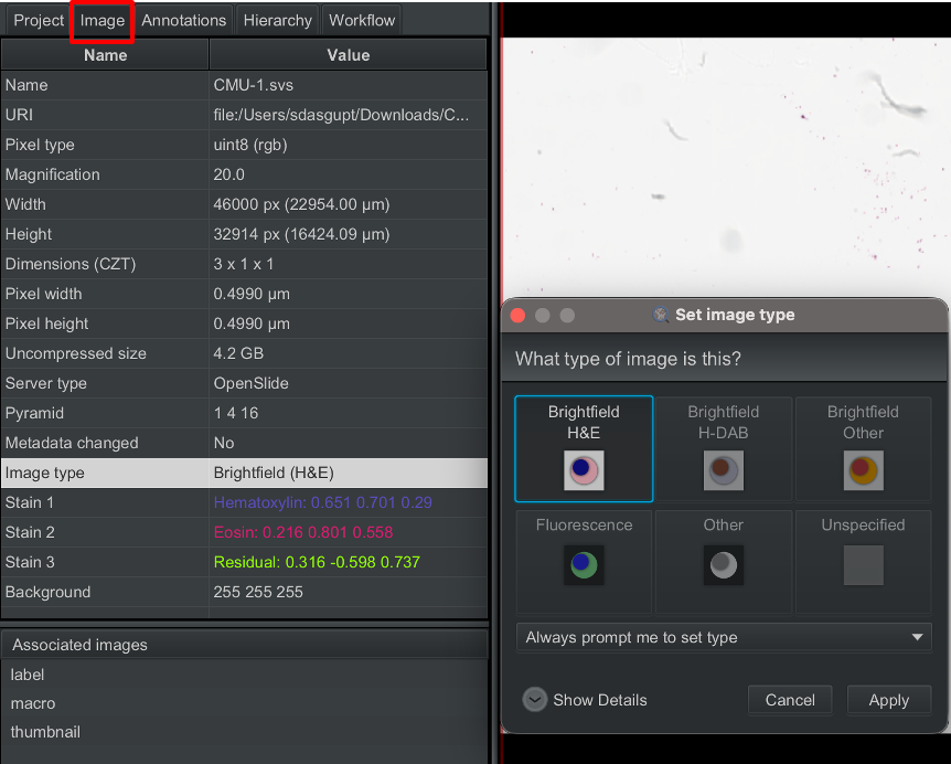
You will be prompted to set the image type, e.g. Brightfield (H-DAB), Brightfield (H&E), Fluorescence etc. when you add an image to a project.

You can always change this by clicking on Image in the analysis pane, and then Image type. The options for setting the image type will appear in a separate window.

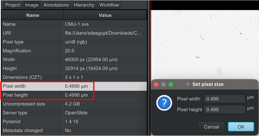
It is also important to correctly set the pixel size. QuPath does this automatically when the image is loaded, but you can also set this manually by clicking on Pixel width or Pixel height entering the desired values.

2.1.5.2 Separate stains

The first step to separating the stains in the image is to set the image type accurately, as described in the section above. For brightfield images, QuPath separates the stains by using color deconvolution method introduced by Ruifrok and Johnston. Please make sure to check out the QuPath docs to learn more about color deconvolution in QuPath.

We will next follow the steps described below to set up the stain vectors. This is an important step because if the stain vectors are inaccurate, steps that rely on color deconvolution, such as cell detection, may perform poorly because the signals from different stains may not be properly separated.

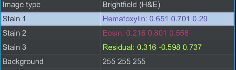
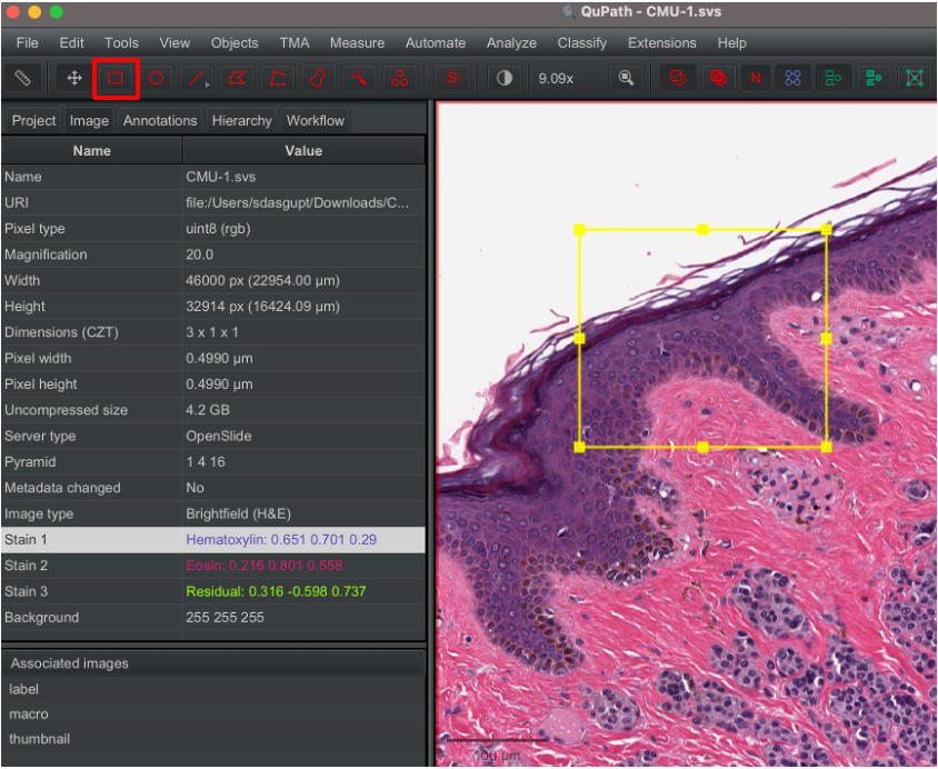
1. Since you set the image type as Brightfield (H&E), you would be able to see the names of the stains, Hematoxylin and Eosin, under the Image tab.

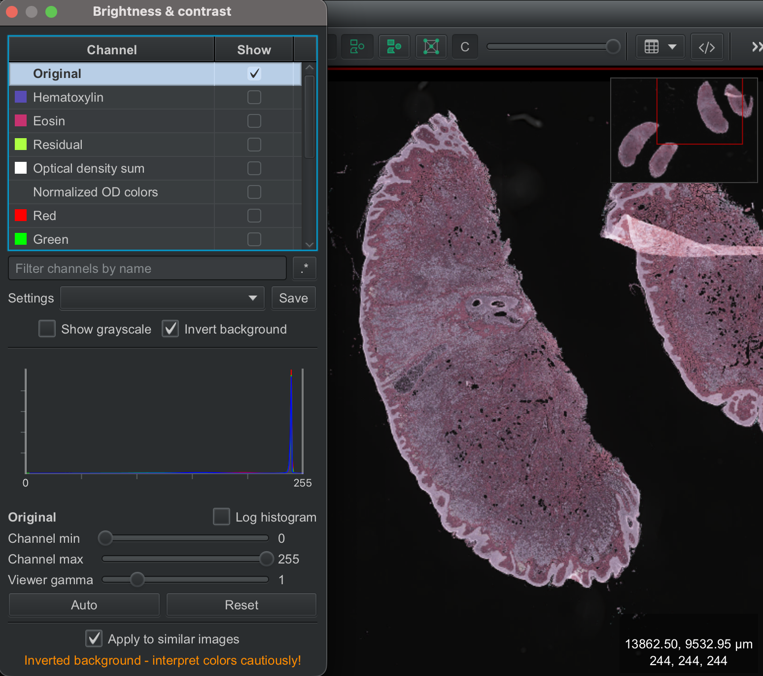
2. You can also visualize the different stains in your image individually by clicking View --> Brightness and Contrast.

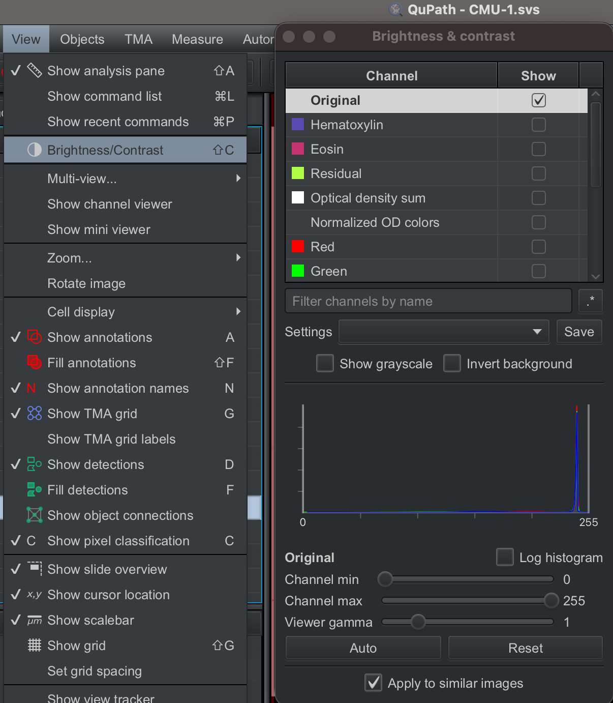
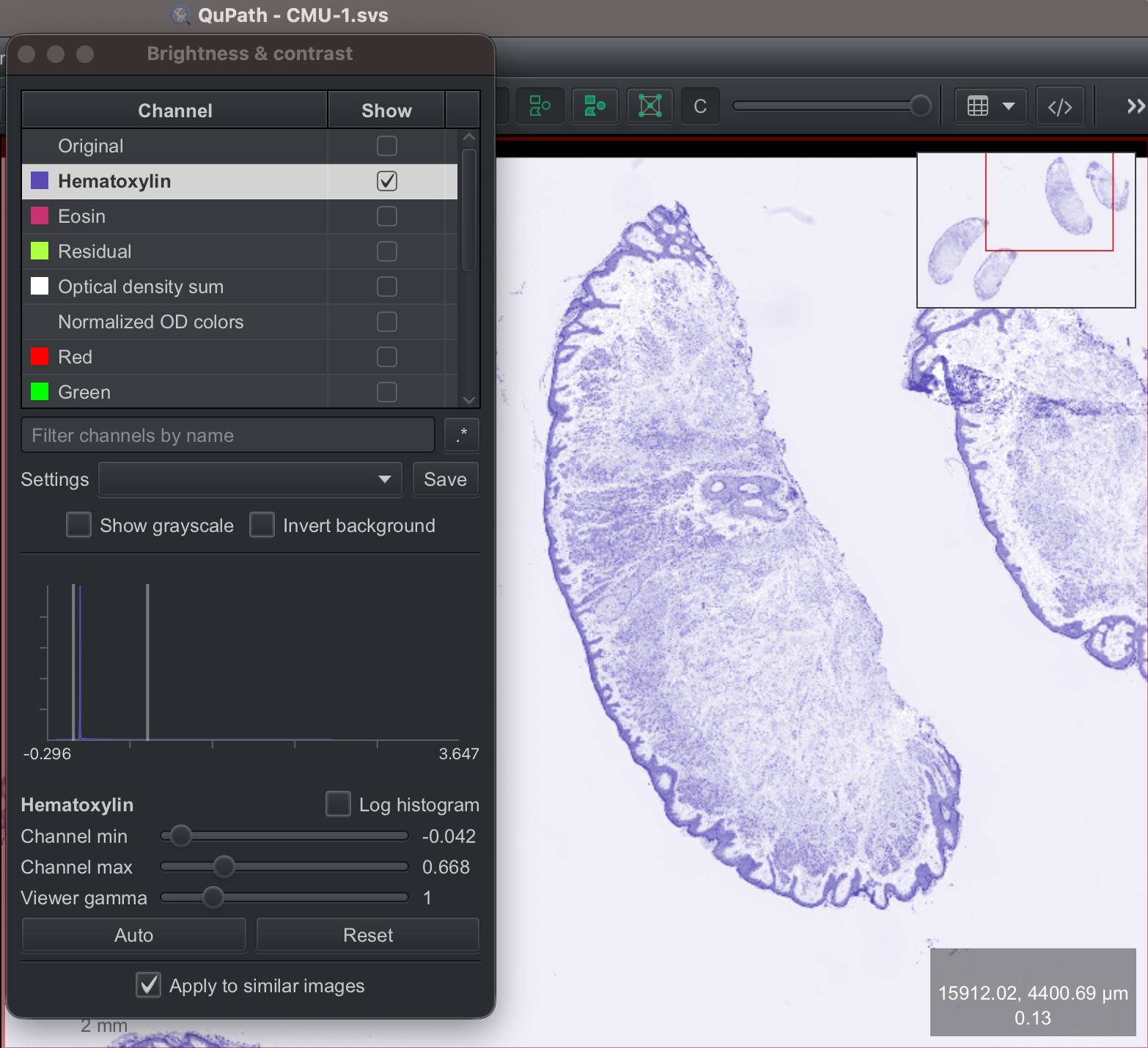
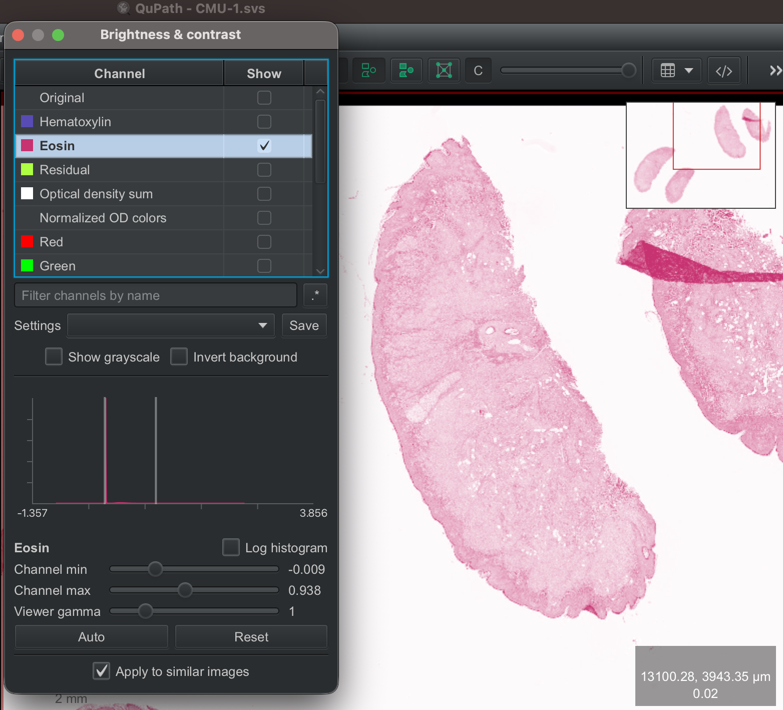
The Brightness and Contrast button provides many helpful options,e.g.,

Viewing one stain at a time

Viewing the image in grayscale

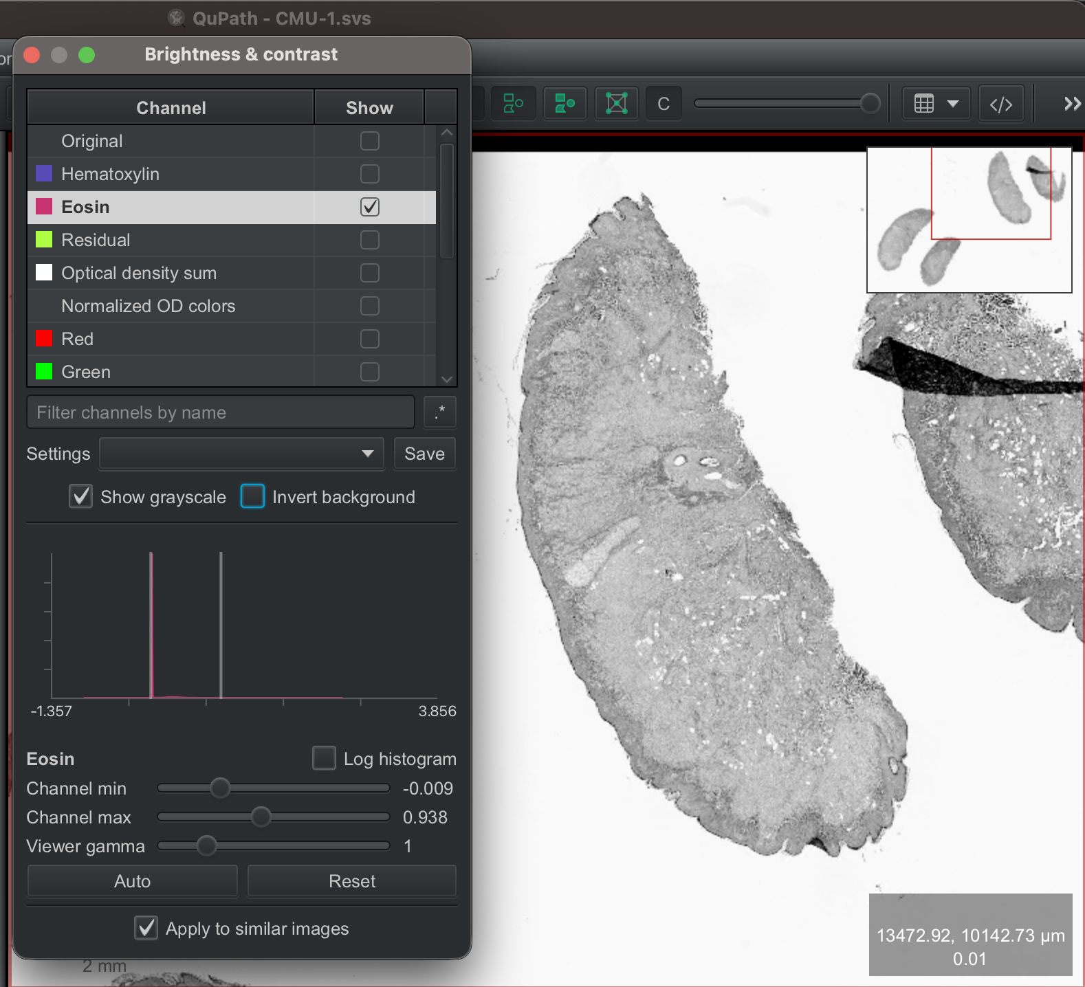
Inverting the colors of the image

3. Next, we annotate an area of the image that has clear examples of the stains that we want to separate, along with an area of the background. For this, we use the rectangle annotation tool (red box).

We then click on Analyze --> Estimate stain vectors and then Yes

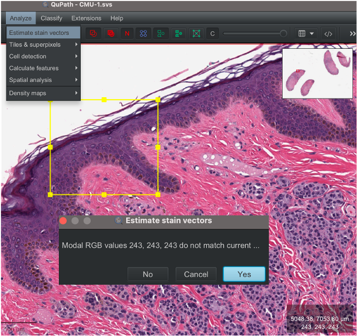
QuPath will then show the 3D relationship between the red, green, and blue pixels in the image as 2D scatterplots, and also indicates the existing stain vectors with colored lines.

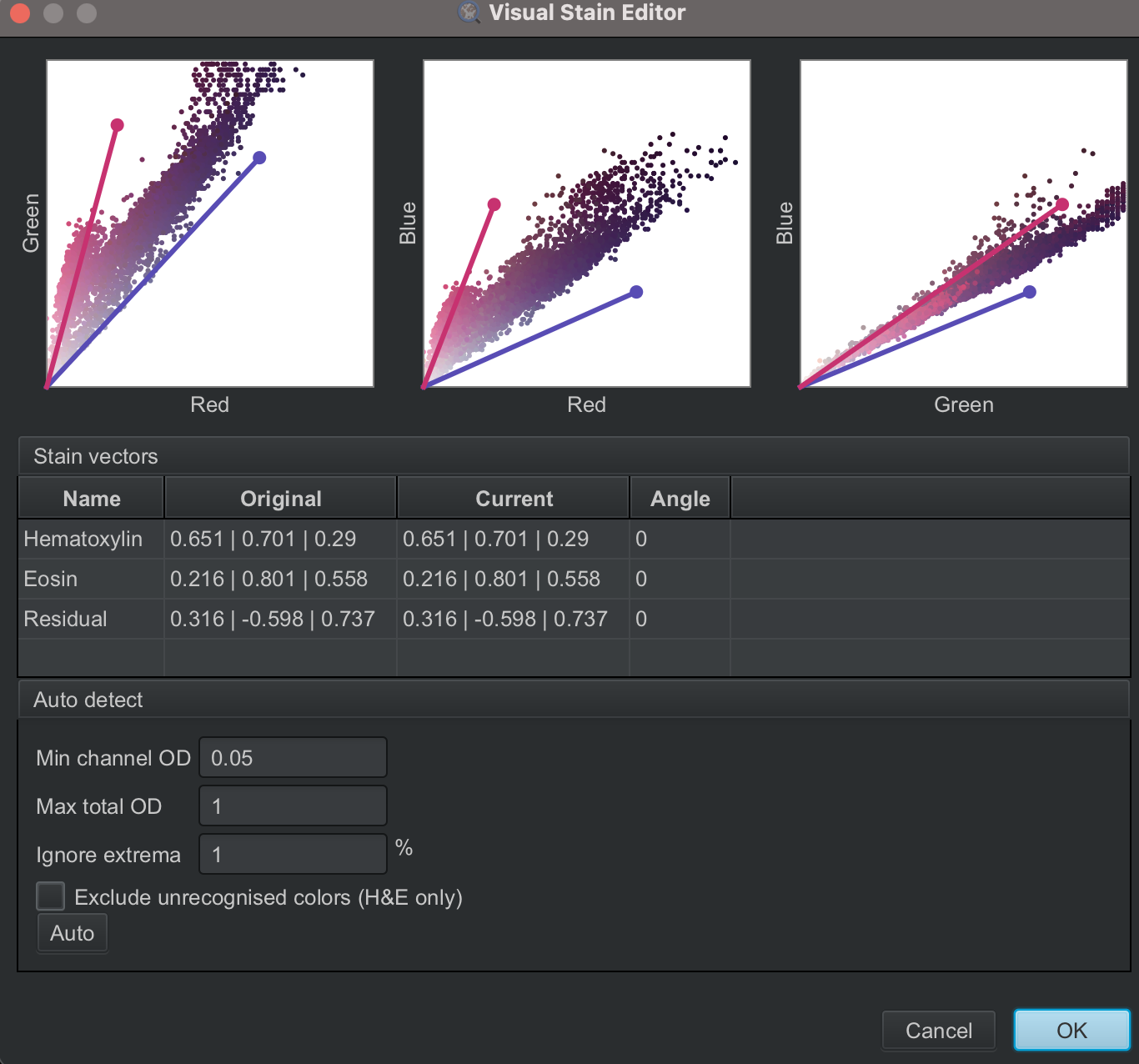
These scatterplots help assess whether the stain vectors match the pixel colors in the selected region. Ideally, the vectors should closely align with most of the scattered points.

If the vectors are not well aligned, the Auto option can estimate improved stain vectors from the selected region. However, unexpected colors, such as greenish pixels, can distort the estimate. In such cases, adjusting parameters like Exclude unrecognised colors (H&E only) can help remove irrelevant colors and produce more reliable stain separation.

2.1.6 Annotate images

---

Annotations in QuPath can have many applications. Common use cases include measuring lengths or areas, defining specific regions where analysis should be applied, such as cell detection, as well as selecting representative areas for training a classifier. For this tutorial, we will learn to annotate some regions interest (ROI) in an image and perform and export measurements from these ROIs.

2.1.6.1 Draw annotations

Annotation objects can be created by drawing specific shapes on the image, using the (1) rectangle, (2) ellipse, (3) line, (4) polygon, or (5) polyline tools. The (6) brush tool and the (7) wand tool are particularly handy for drawing custom shapes. All of these tools can be applied by selecting the tool, clicking on the image, and dragging the mouse. For the polygon tool, the shape can be completed by releasing the mouse or by double-clicking where the final point should be.

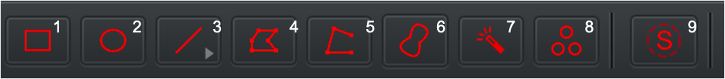
⚠️ Tip: The wand tool is very helpful for making precise annotations around tissue boundaries.

The (9) selection tool converts the annotation tools into tools for selection. This is helpful for selecting multiple annotated regions with a single click and drag. Clicking on the selection tool changes the annotation tool icons into their dashed versions.

Annotations can be deleted by selecting the annotation and pressing Delete on the keyboard, or right-clicking on the annotation and selecting Delete object. If you make a mistake while annotating with the brush or wand tool, simple press Option and click and drag your mouse to erase the incorrectly annotated area. Right-clicking on an annotation “locks” it, and prevents it from getting accidentally deleted.

Make sure to explore some of these annotation tools and draw different shapes and sizes on the image!

2.1.6.2 Set annotation properties

QuPath allows you to make annotations of different classes - these classes depend on the image you are working with and your biological question. For example, if you are working with images of kidney tissue, these classes can be different structures you have annotated in the image and want to analyze further, e.g. glomerulus, tubules etc. Or, if you are working with images of diseased tissue, these can be tumor area / abnormal area or normal / healthy area and so on.

We will now create some annotations of a particular class and set the properties of these annotations.

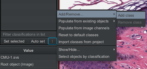
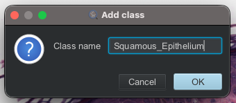
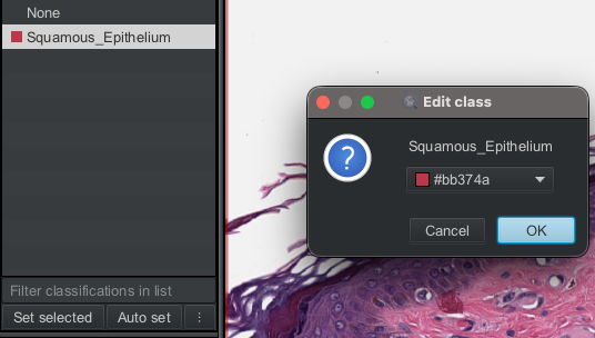
1. Create an annotation class by clicking on the three dots next to Auto set under the Annotations tab in the Analysis pane. Then click Add/Remove --> Add class. A window will open where you can enter the name of the annotation class; we will enter Squamous_Epithelium.

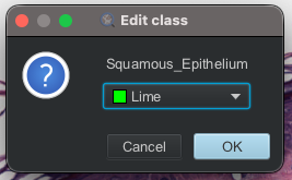
2. This new class of annotation will appear in the analysis pane. If you like, you can double-click on the annotation and select a different color for your annotation by clicking on the drop-down – I have changed the annotation color to Lime.

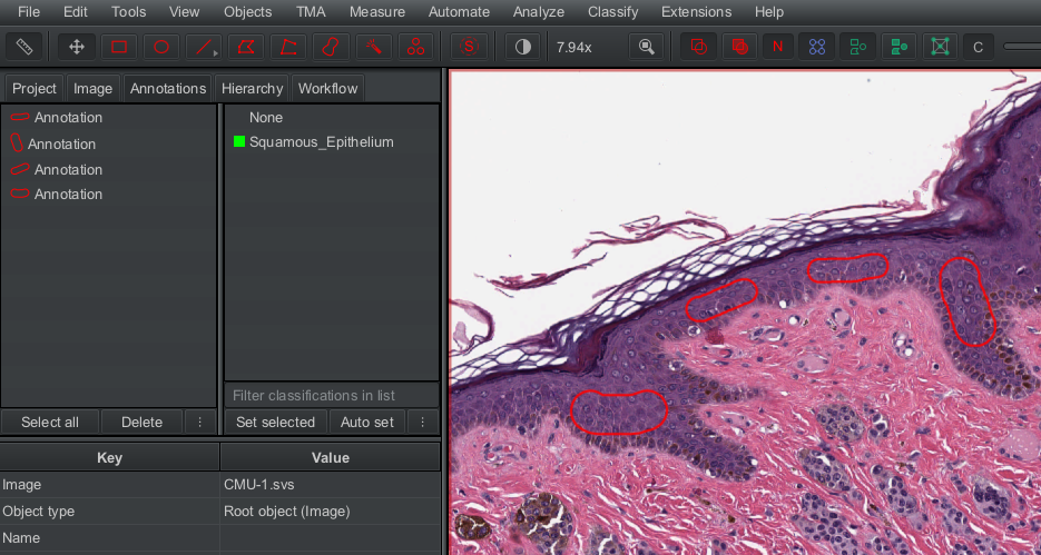
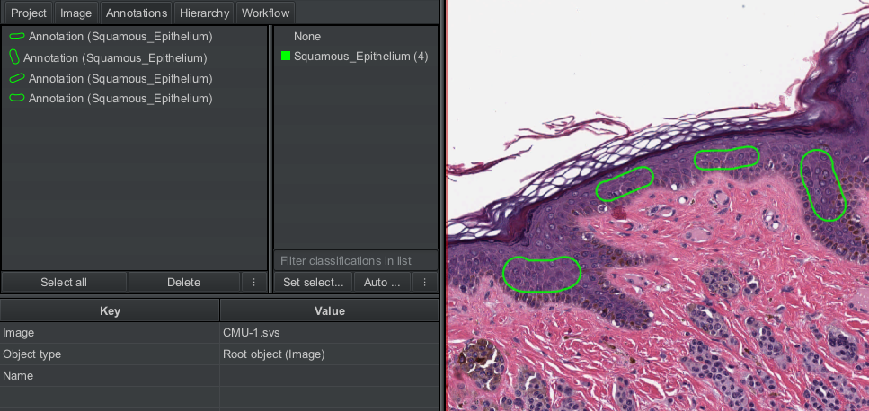
3. We will now draw some annotations on the squamous epithelial lining of the tissue. You can use any tool to do this; I have used the brush tool. You will see the list of annotations appear in the analysis pane. We will now assign a class to these annotations.

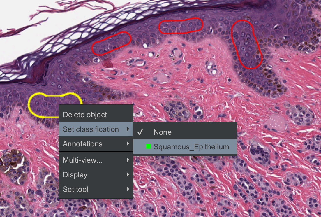
4. Double-click on any annotation – you will see the outline color change to yellow, which means you have now selected the annotation. If you now right-click on the annotation, you will have the option to assign it a class. Click on Set classification --> Squamous_Epithelium. You can do this one-by-one for each annotation. You will see now the thumbnails of the annotations will have a class next to them, and the class Sqaumous_Epithelium has a number next to it indicating the number of annotations that exist in this class.

⚠️ Tip: To assign a class to multiple annotations in one step, select all the annotation thumbnails in the analysis pane. This will select all the annotations in the viewer. You can then right-click on any annotation and set the classification as described above.

5. Now we will set the properties for each annotation, i.e., assign a unique label to each annotated area of the class Squamous_Epithelium.

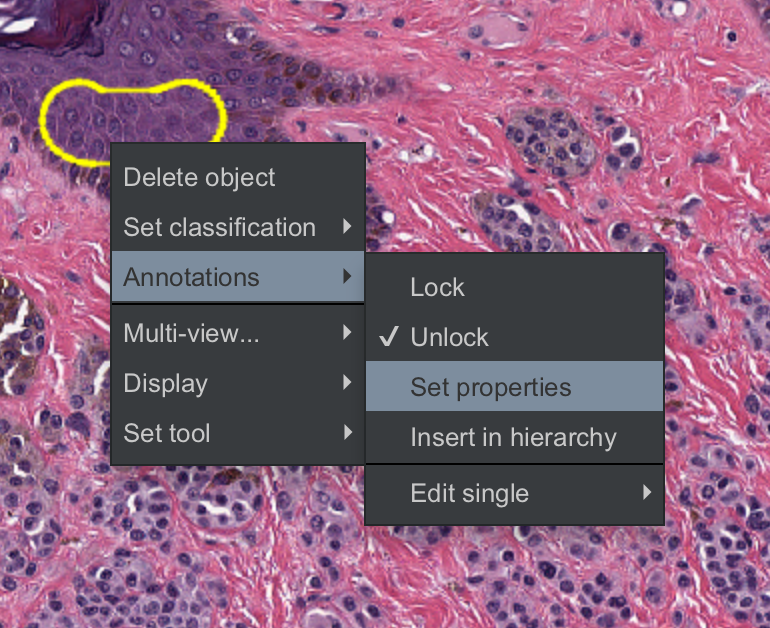
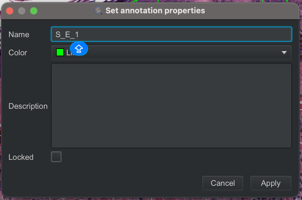
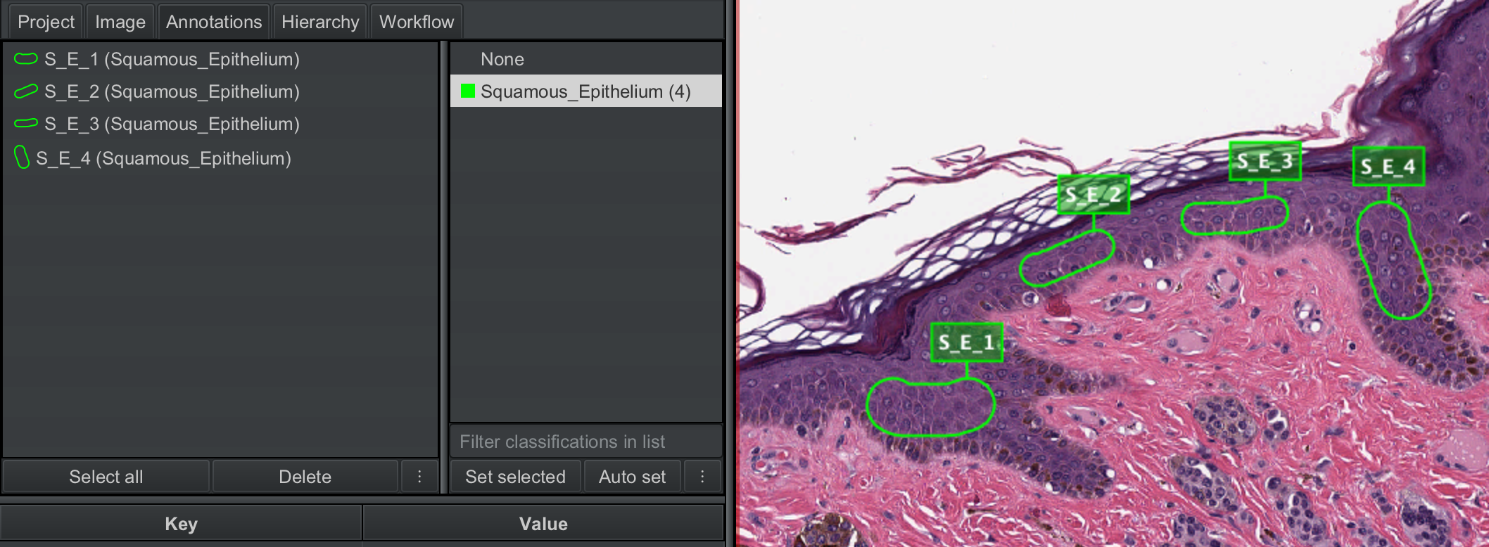
   To assign labels, we double-click on each annotation, select Annotations --> Set properties and enter a name, You can also add a description if you like. I have named the annotations S_E_1 (abbreviation for Squamous_Epithelium) through S_E_5. You will notice that the annotation labels now appear next to the annotation thumbnails in the analysis pane, and you can also visualize these labels in the viewer.

Why do we do this step?

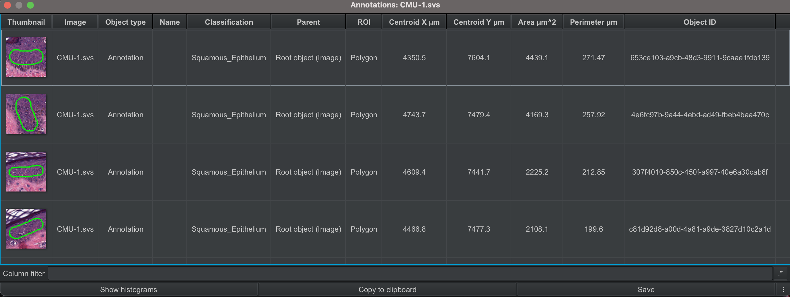
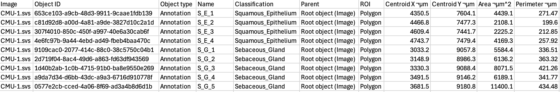
If we do not assign unique labels to each annotation, when we perform measurements and export the data, we will not be able to tell exactly which annotation the measurements belong to. This is because, the exported measurement table will look like the figure below, where each row has the measurements for each annotation, but without labels, so we cannot look back at the image and map the measurements back to the annotations.

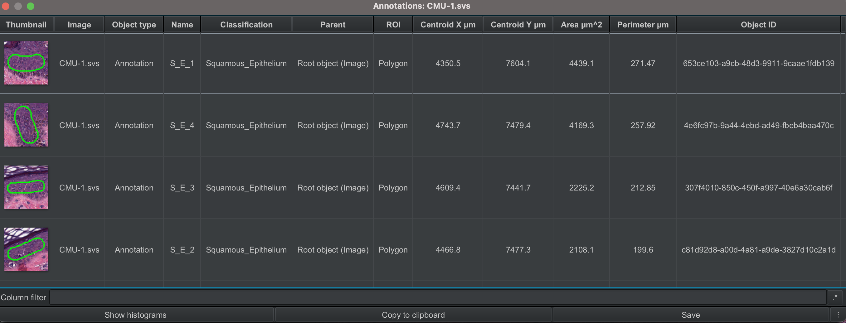
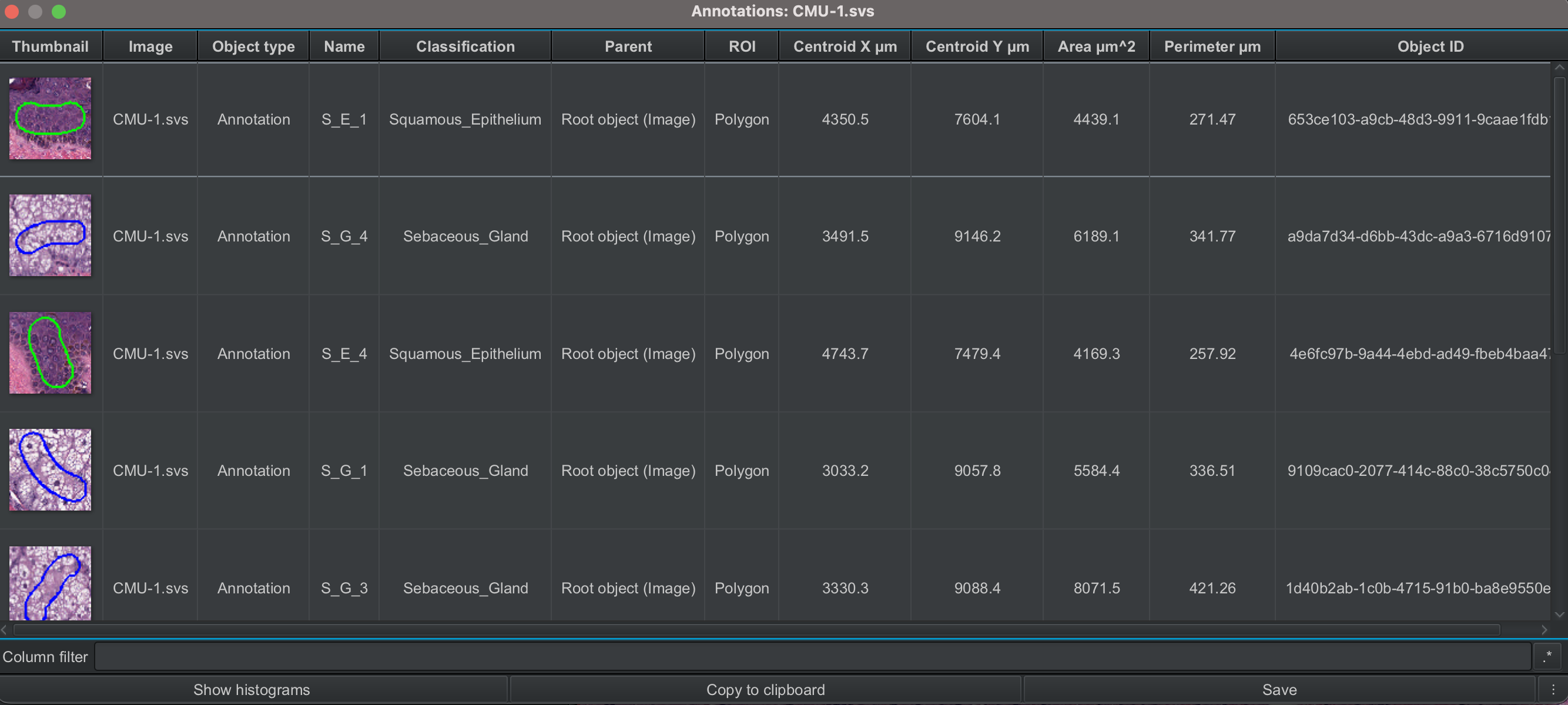
However, if we assign unique labels to the annotations, the exported table will include these annotation labels, as you can see in the figure below, and these labels can also be visualized in the viewer. This allows us to precisely map the measurements back to the annotations in the image.

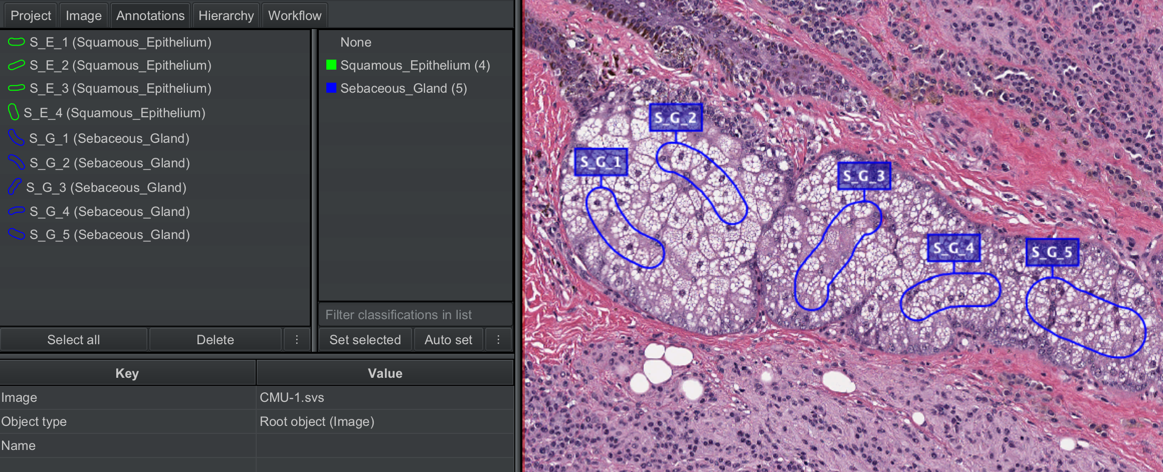
Now try making annotations of a different class with different names as shown in the figure below!

⚠️ Hint: You will pretty much use the same steps as described above!

2.1.7 View and export annotation measurements

For every annotation created on the image, QuPath performs some measurements such as area, perimeter, X and Y co-ordinates. There are several ways of viewing these measurements.

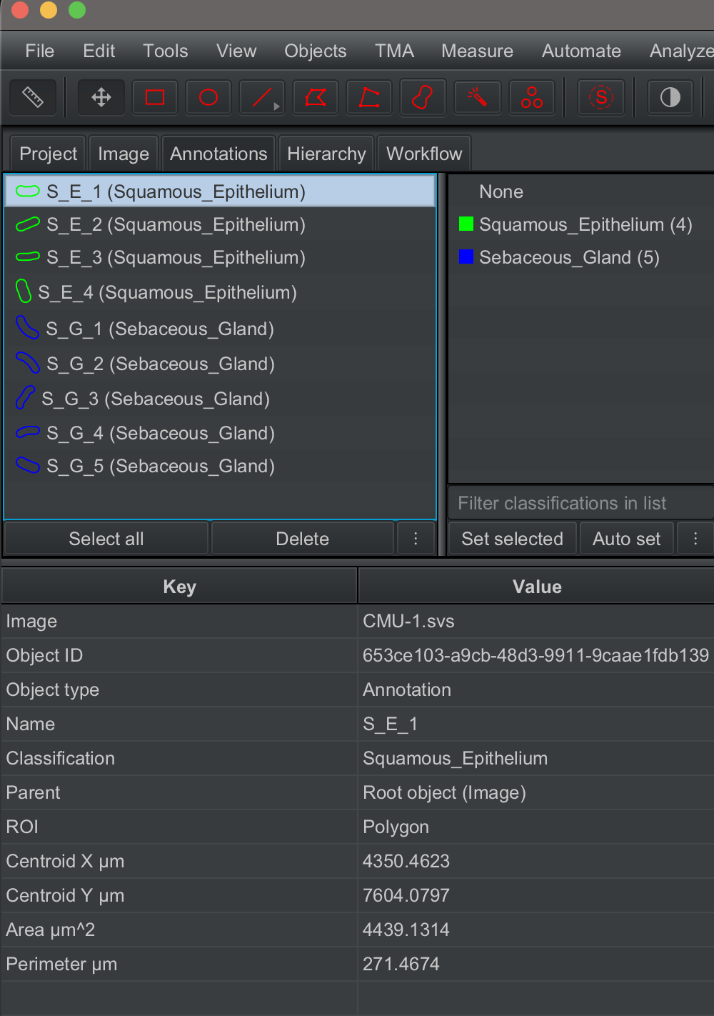
• If you click on the thumbnail of any annotation under the Annotations tab, you will see the measurements that QuPath has made for that annotation will populate the table below.

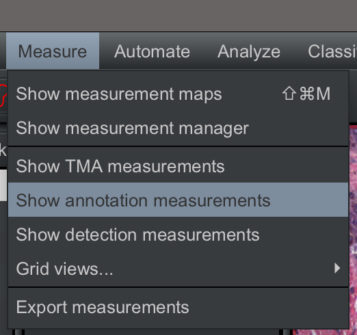
• You can also view the per-annotation measurement table by clicking on Measure --> Show annotation measurements

To export the measurements, you can click on Save in the measurement table. This will allow you to export this table as a .txt file.

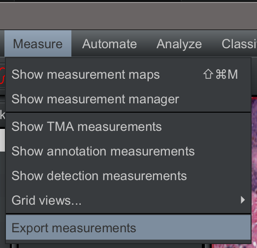
Alternatively, you can click on Measure --> Export measurements. But before you do this, make sure you have saved the changes by clicking File --> Save.

This will open a window where you will need to set the following:

• Choose the image for which you want to export the measurement. In this tutorial, we have only one image, and select this by clicking on the arrow (red box)

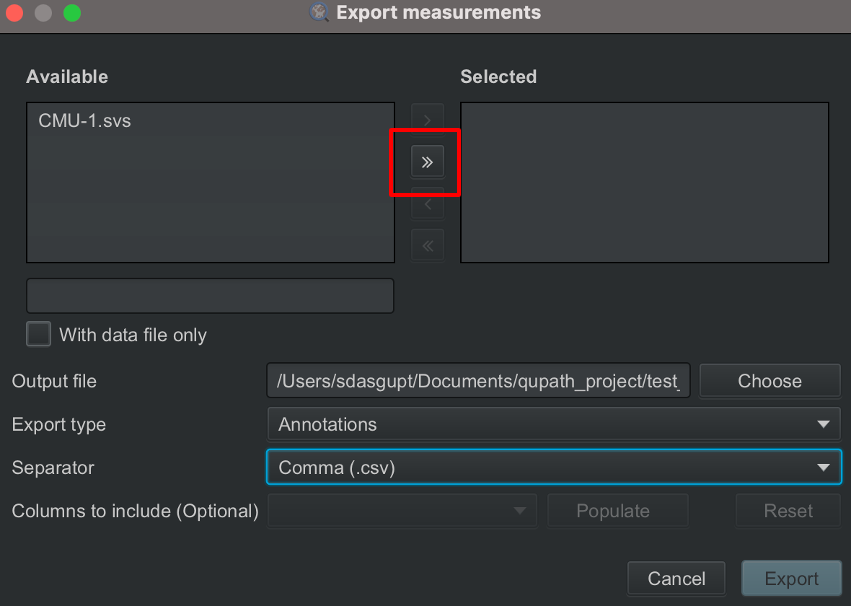
You will see the selected image move to the box on the left.

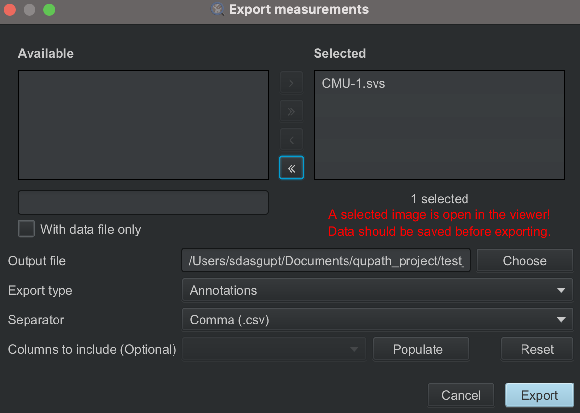
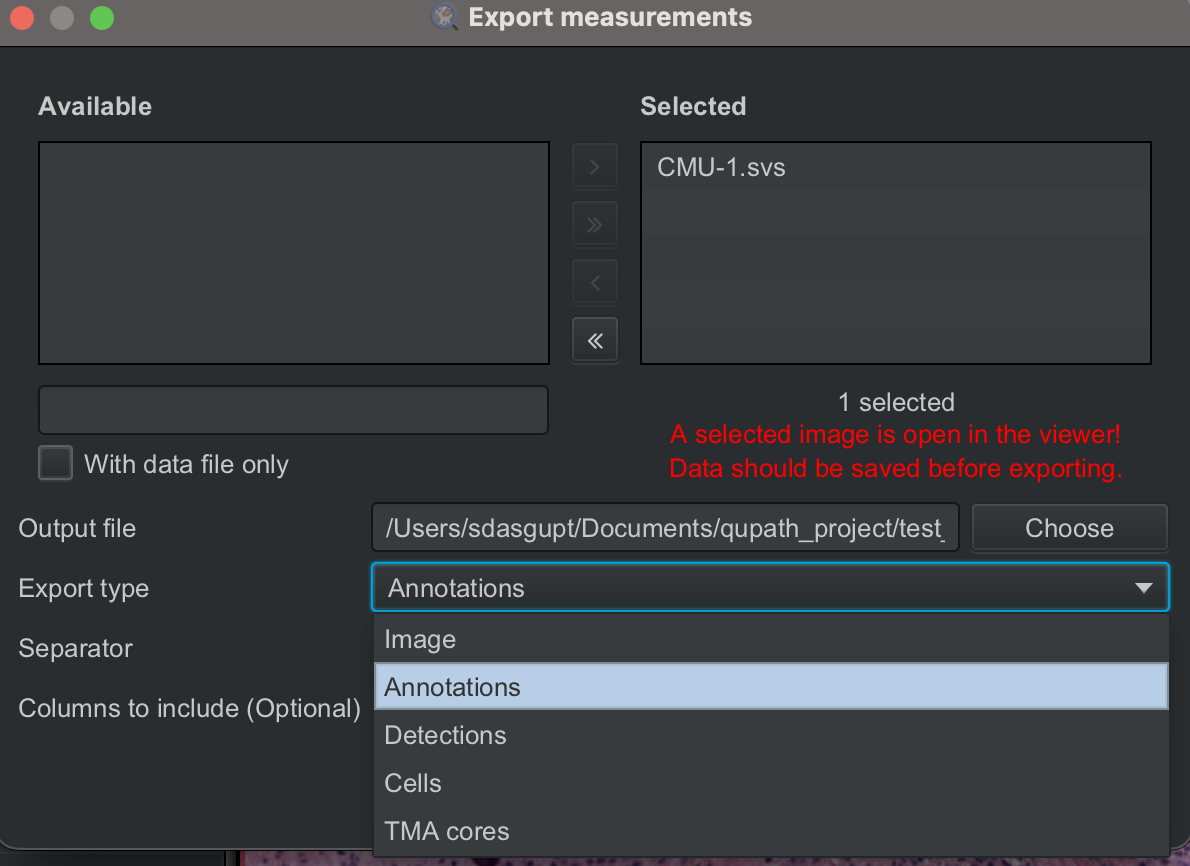
• Click on Choose to set up the name of the file and the location where the file should be saved.

• Select the type of measurements you want to export, i.e., image, annotations, detections etc. We want to export the annotation measurements.

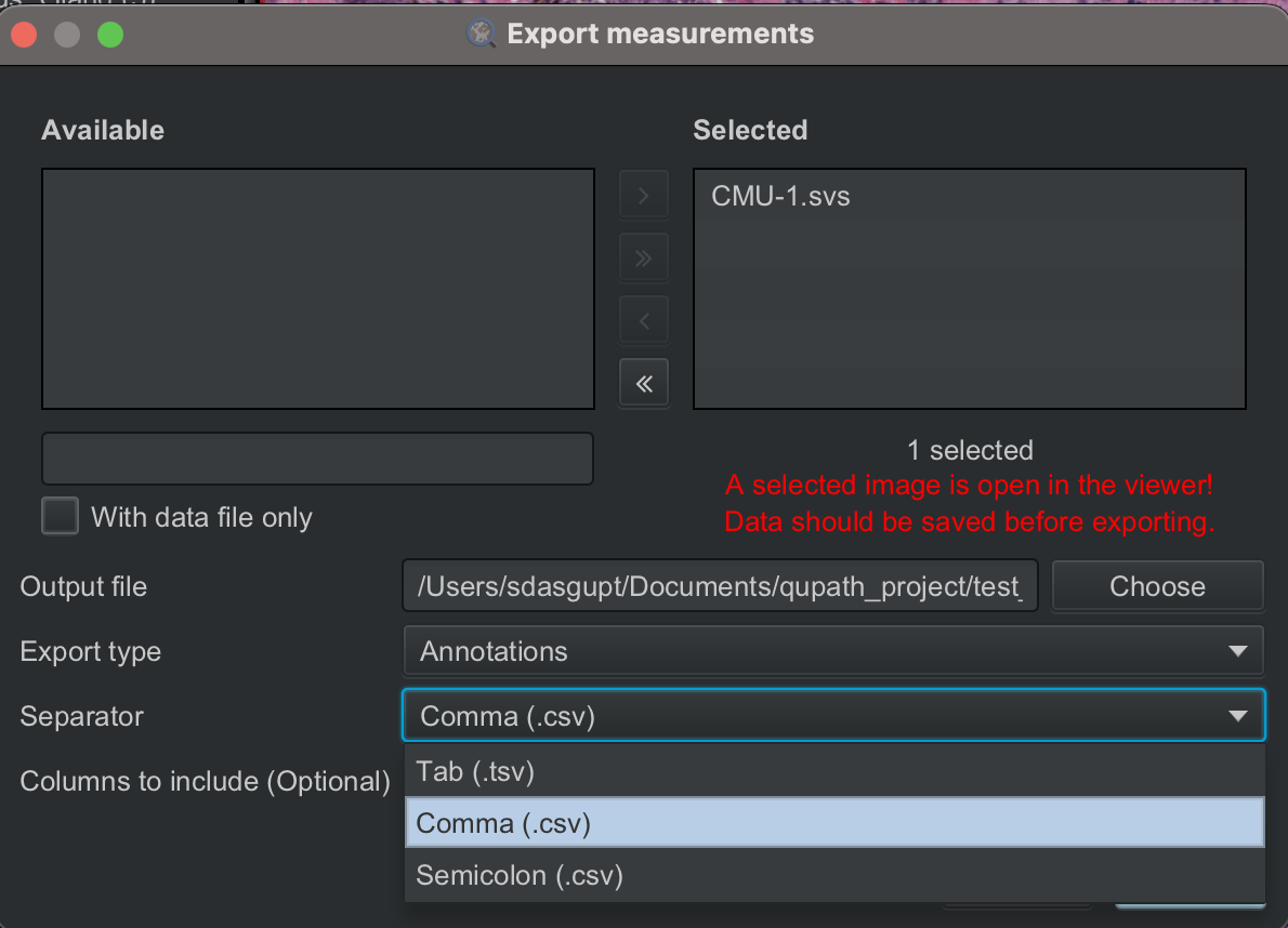
• Select whether you want the measurements exported to a .csv or .tsv file. Let us export the measurement to a .csv file.

• Then, click Export. QuPath will export the data into a .csv having the name that you set and the location that you selected. For this tutorial with the annotations I made, the file looks like this opened in Excel.

If you want to get a bit more practice with steps 2.4 to 2.7, feel free to download a couple more H&E images from here and add to your current project!

2.2 PART II

For this part of the tutorial, we will learn how to detect positive cells, meaning cells that show staining, by analyzing a tissue section immunohistochemically stained with a nuclear marker. Before detecting positive cells, we will also annotate specific regions of interest within the tissue section, allowing us to link individual cell measurements back to the tissue regions where those cells are located. We will be working with the OS-2.ndpi image.

2.2.1 Create a QuPath project

---

We will create a new QuPath project and add the OS-2.ndpi image to the project, following steps detailed in 2.1.2 and 2.1.3. I have named the project qupath_project_IHC; you can name the project according to your preference. We will set the image type as Brightfield (H-DAB).

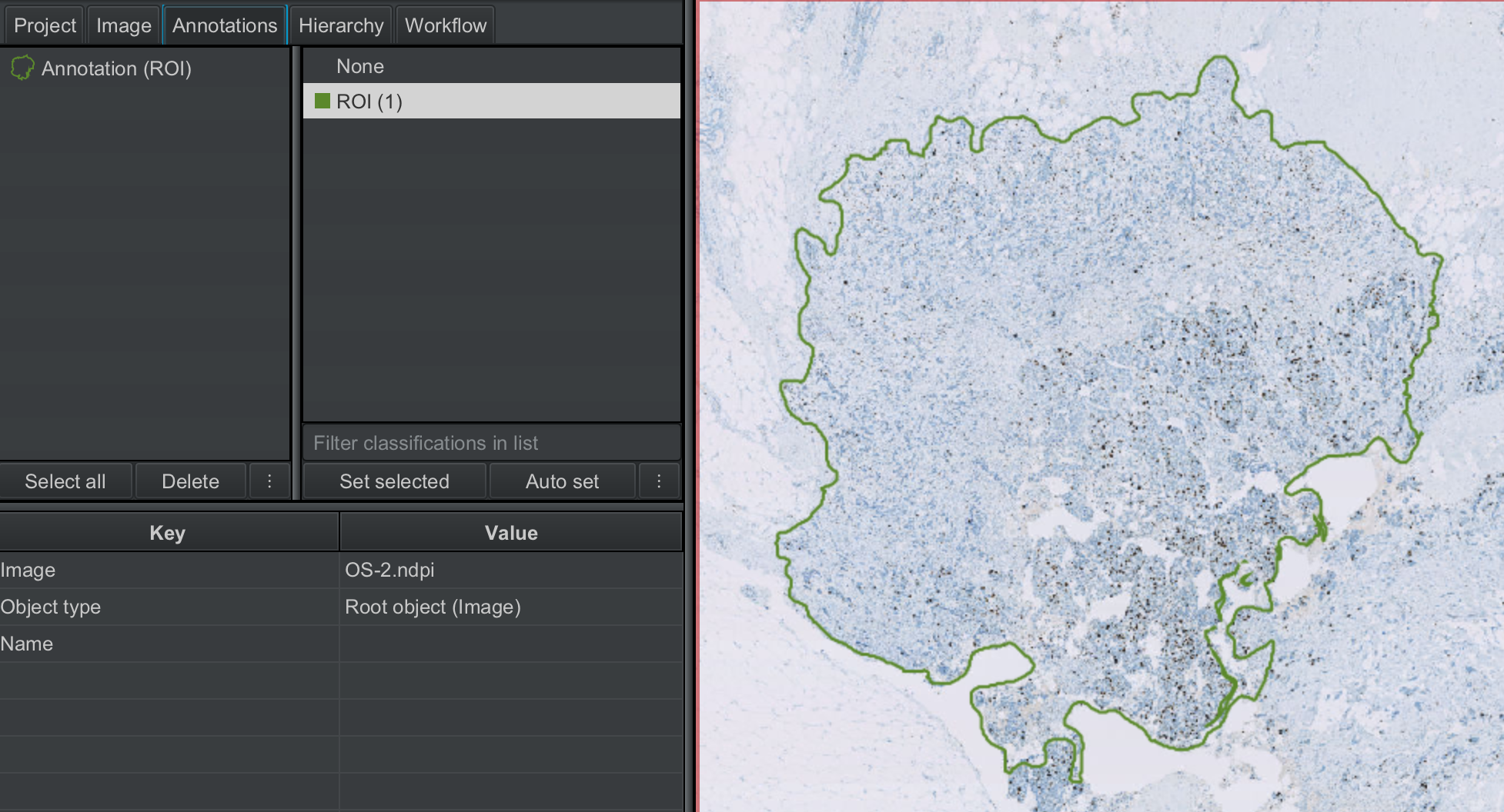
2.2.2 Annotate the region of interest

---

Let us first create a new class of annotations called ROI (region of interest), following steps detailed in 2.1.6. Next, using the wand tool (or any annotation tool of your preference), let us annotate a specific part of the tissue. This is the part of the tissue where we want to detect the cells.

2.2.3 Perform positive cell detection

---

We will now detect the cells in ROI to perform measurements on these cells, and also to classify these cells as positive or negative for the nuclear marker.

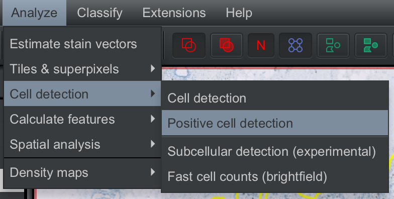
1. Select the annotation ROI; the color of the outline will change to yellow.

2. Click on Analyze --> Cell detection --> Positive cell detection

3. This will open a window where you can set up cell detection parameters, e.g. setting the minimum and maximum area of the cells, intensity threshold, and so on. Also, note that QuPath detects cell outlines by expanding the nucleus outlines by a fixed distance; this can also be set at this step. Since we are categorizing cells as positive or negative based on a nuclear marker, we use Nucleus: OD DAB mean as the score compartment to set the intensity threshold.

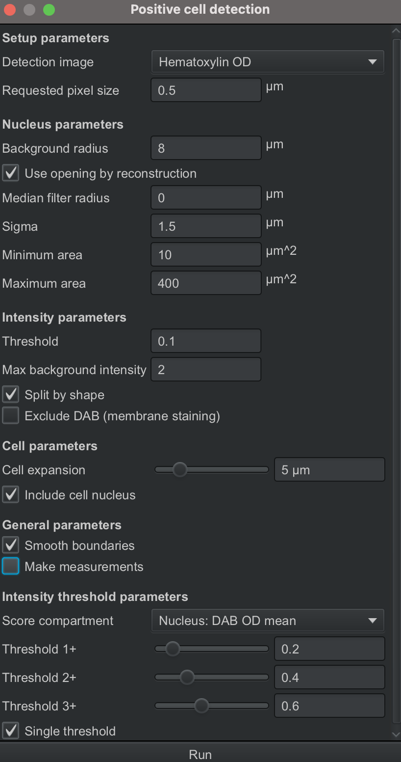
For the purpose of the tutorial, we will use the default parameters and hit Run, and QuPath will start detecting the cells.

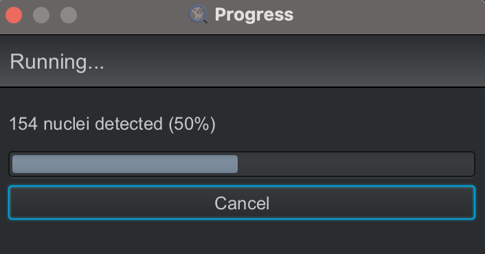
When QuPath finishes, the cell (detections) outlines will appear on the image within the annotated area (ROI) where the detection was run, and the number of detections will be updated in the analysis pane next to the annotation thumbnail. The positive cells are outlined in red and negative cells in blue. The analysis pane now also shows the number of positive and negative cells detected.

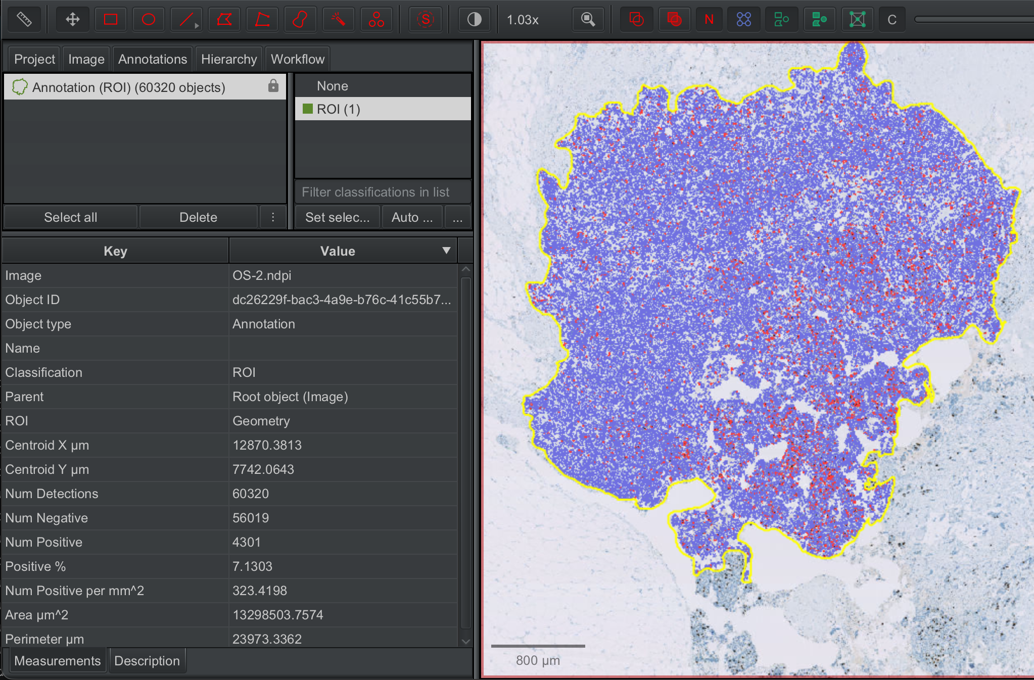
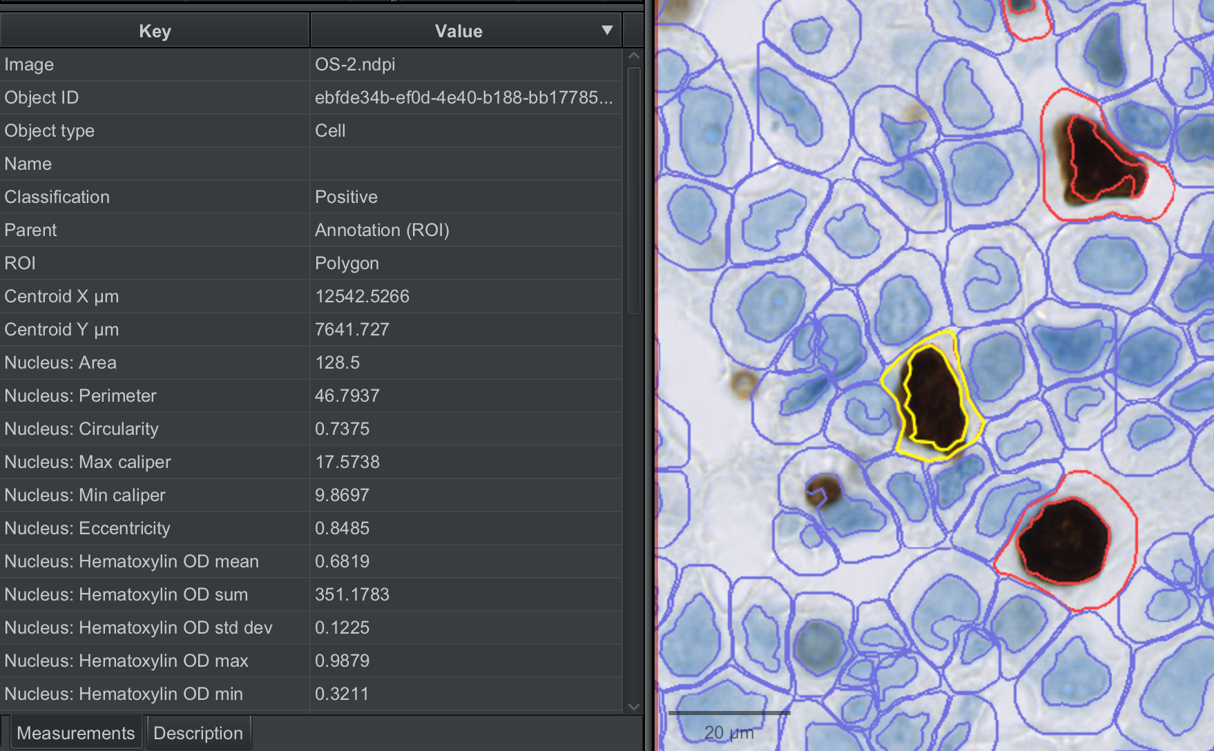
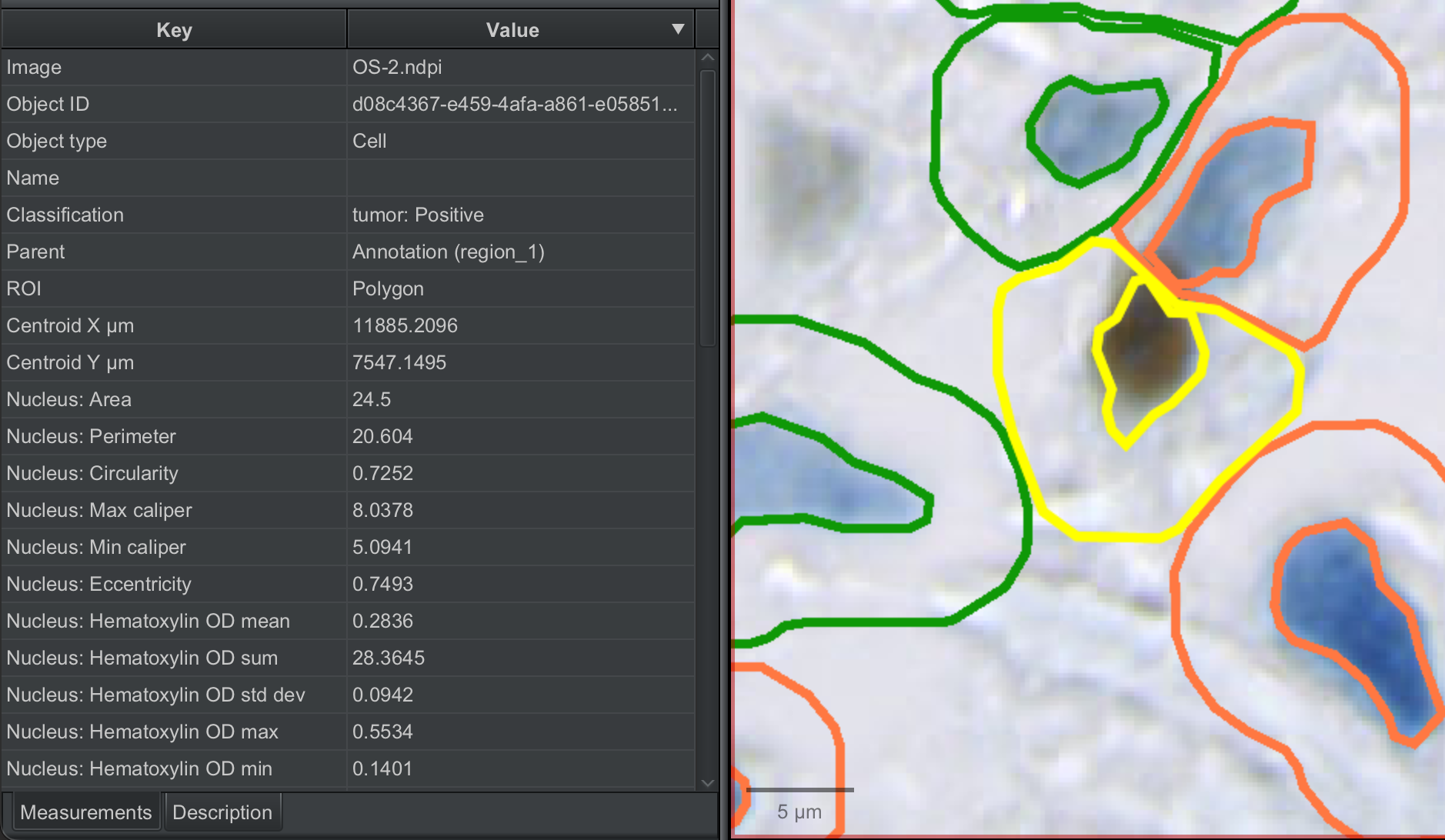
If you zoom into the image and click on any detected cell, you will see the analysis pane will be populated with the measurements that were performed on that cell.

⚠️ Hint: You can turn annotations and detections on and off in the viewer by clicking A and D on the keyboard respectively!

2.2.4 Annotate areas within the region of interest

---

If you click on any of the detected cells, you will see in the analysis pane that the Parent of this cell (detection) object is Annotation (ROI) Let’s say, we are interested in comparing features of cells that are located in two specific areas within this ROI, e.g. region_1 and region_2. In that case, we would want the detected cells to also have these additional annotation labels, i.e region_1 and region_2.

To achieve that, we will perform the following steps:

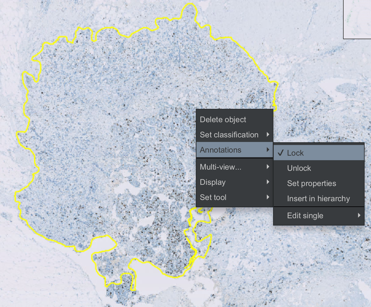
1. Temporarily, turn off the cell outlines by clicking D or unchecking Show detections under View

2. Lock the annotation ROI. Right-click on the annotated area, select Annotations --> Lock

3. We now annotate the addtional areas of interest within ROI. I used the rectangle annotation tool, but any tool can be used.

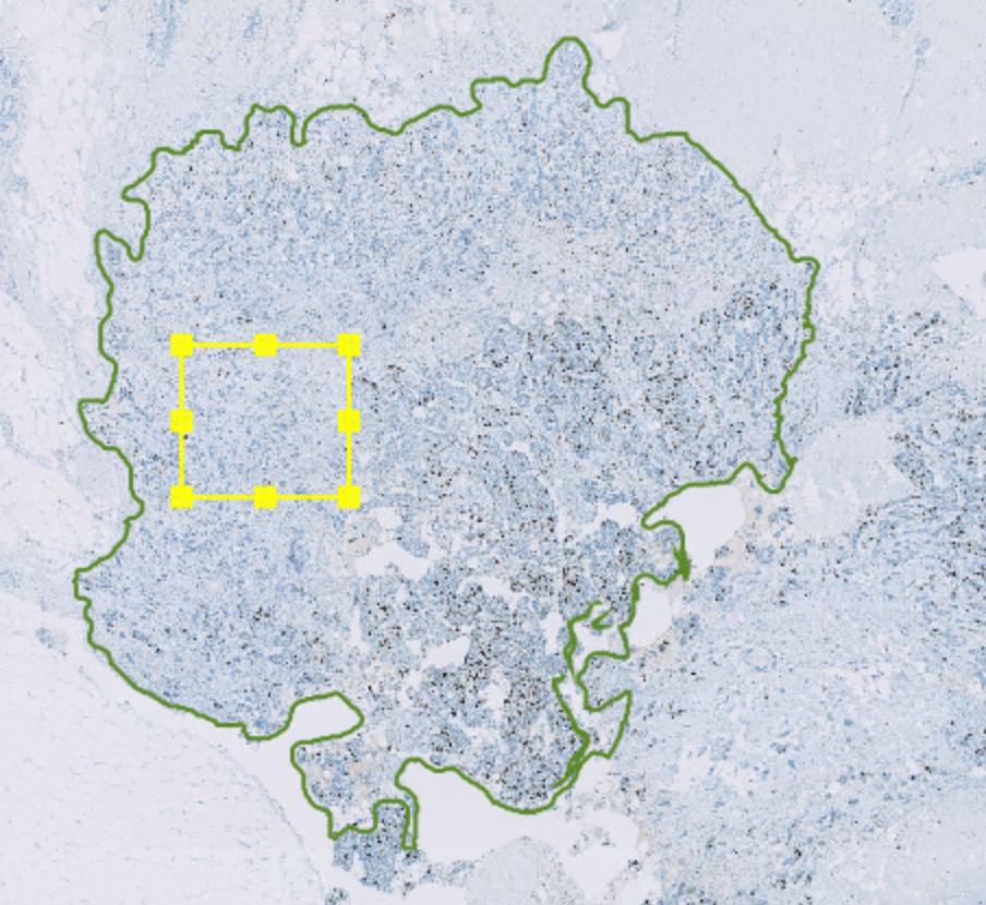
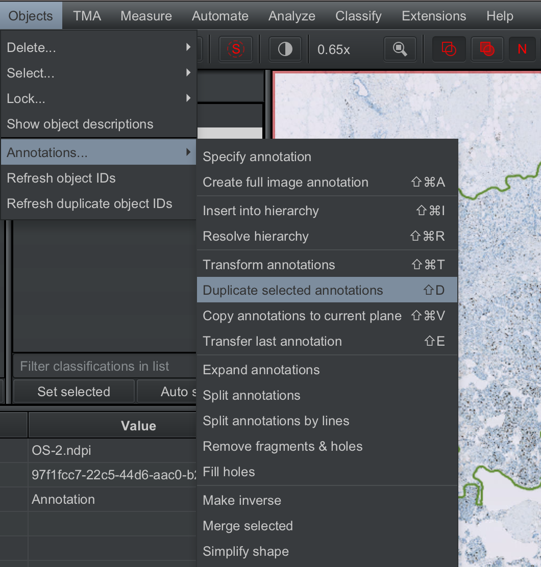
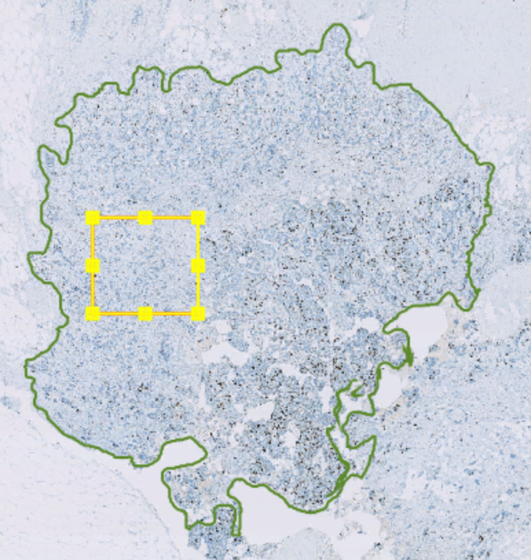
4. To create annotations of the exact same size, I selected the first annotation, and clicked on Objects --> Annotations --> Duplicate selected annotations

5. The duplicated annotation will appear on top of the original annotation. Use the move tool to drag it to the position where you actually want it placed.

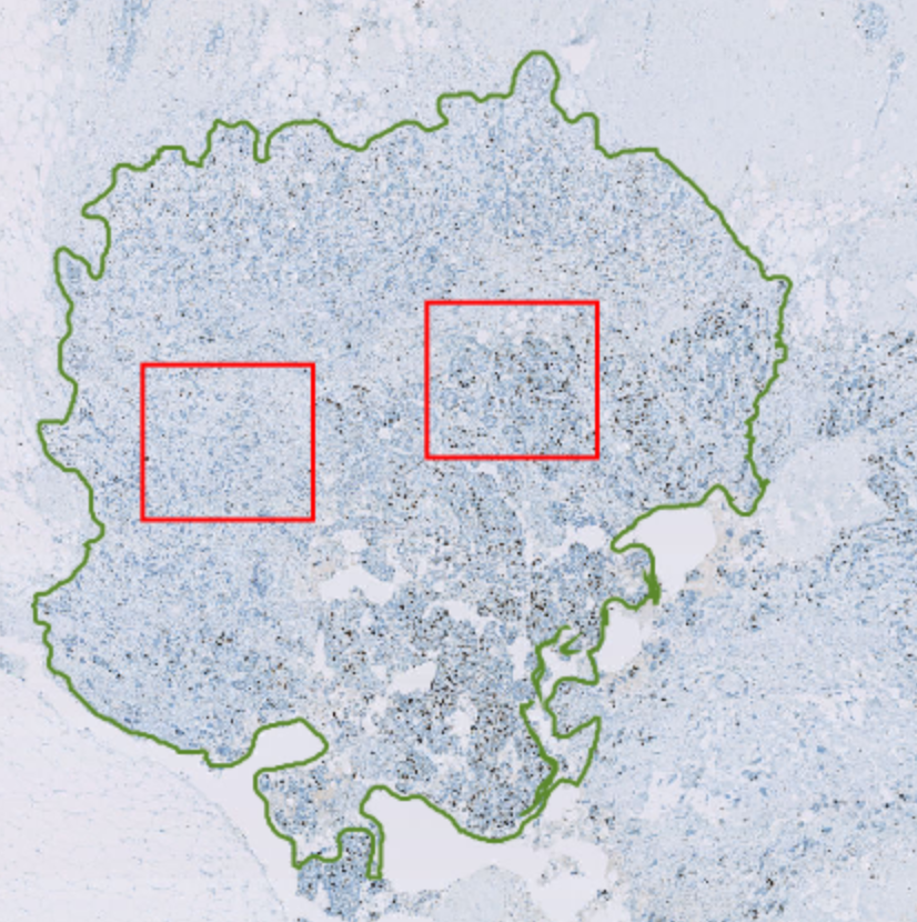
6. Create two new annotation classes region_1 and region_2, as detailed in 2.1.6.2, and set the classifications of the annotations that you made in step 5. Feel free to use any name that you like. In your real analysis, this will be guided by your research question.

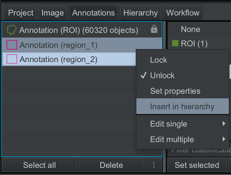
7. Now, we need to let QuPath know that region_1 and region_2 belong to our first annotation ROI. This is called inserting objects into a hierarchy, where annotation objetc ROI will be the root or parent, and annotation objects region_1 and region_2 will be the children. To do this, select the thumbnails for region_1 and region_2 in the analysis pane (shift + down arrow keys), and then Insert in hierarchy.

The analysis pane will now show the number of detections that are present in region_1 and region_2.

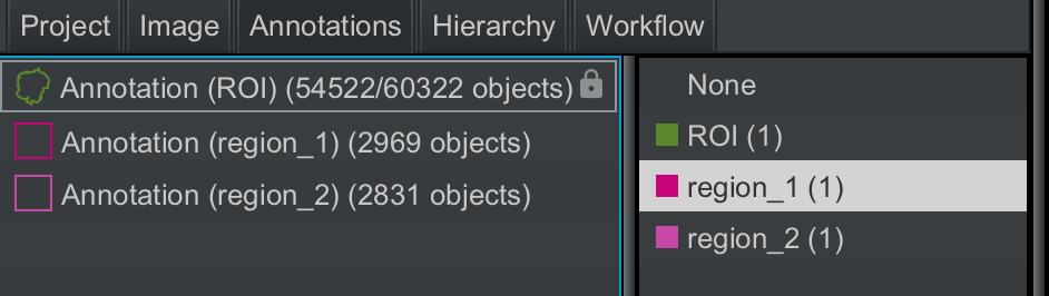
8. Lock the annotations region_1 and region_2.

2.2.5 Create and run object classifier

---

In addition to classifying cells as marker positive or marker negative, it is also possible to classify cells based on their morphological or biological properties. For example, in this tissue section, there are tumor cells and stromal cells. It might be helpful to know how many of the marker positive cells were tumoral and how many were stromal. To achieve this, we will need to perform object classification.

1. Create two new annotation classes - tumor and stroma

2. Manually annotate some tumor and stroma regions within the ROI using any annotation tool of your preference - I have used the brush tool. Try to make sure you draw a comparable number of annotations of each class to avoid any class imbalance.

3. Set the classification of every annotation you draw as tumor or stroma.

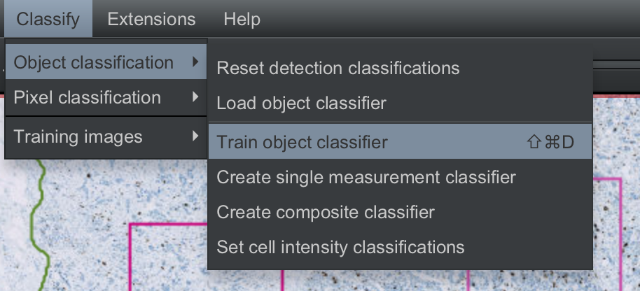
4. Once you are satisfied with the annotations you have drawn, click on Classify --> Object classification --> Train object classifier

5. We will train a Randome trees classifier using all detections and the unlocked annotations (tumor and stroma). QuPath also offers the option of training artifical neural network or K-nearest neighbor based classifiers. These can be selected by clicking on the dropdown next to Classifier.

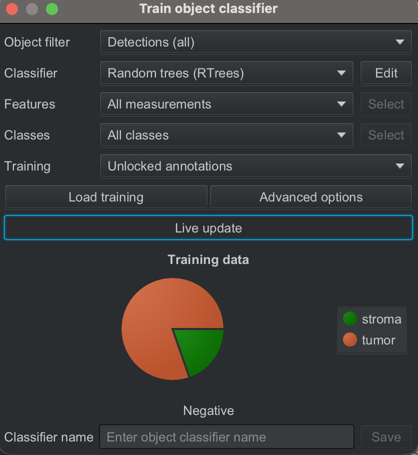
6. Click on Live update to get a preview of the proportion of cells being categorized as tumor or stroma. If this does not match what you would expect from your visual estimate, you can try making more annotations or refining existing annotations to improve the classifier performance. Once you are satisfied with the performance of the classifier, you can give it an appropriate name and click on Save. The classifier will be save in your QuPath project folder.

├── classifiers
│   ├── classes.json
│   └── object_classifiers
│       └── tumor_stroma.json

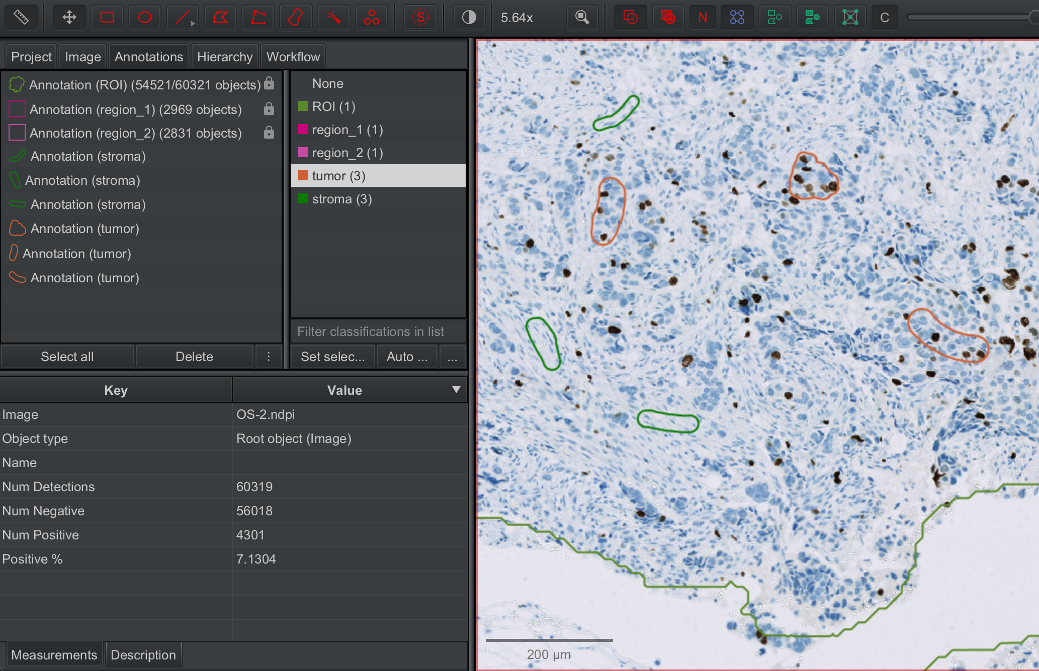
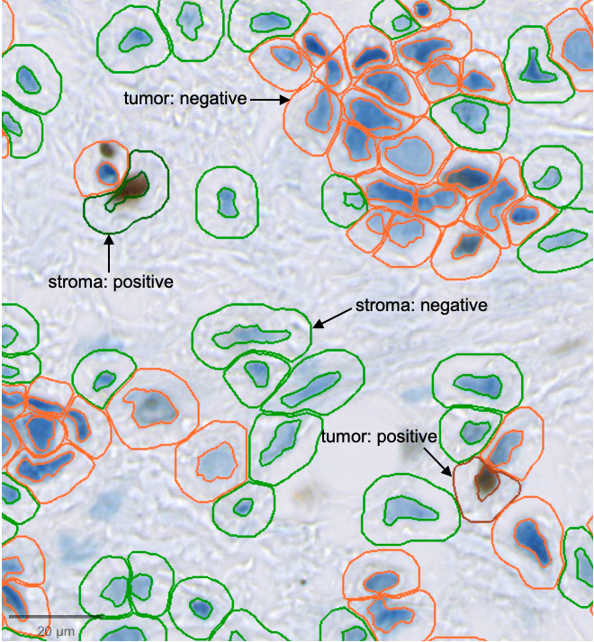
7. All the detected cells will now be classified as tumor or stroma by the classifier you just trained. The cells will also have the classification positive or negative

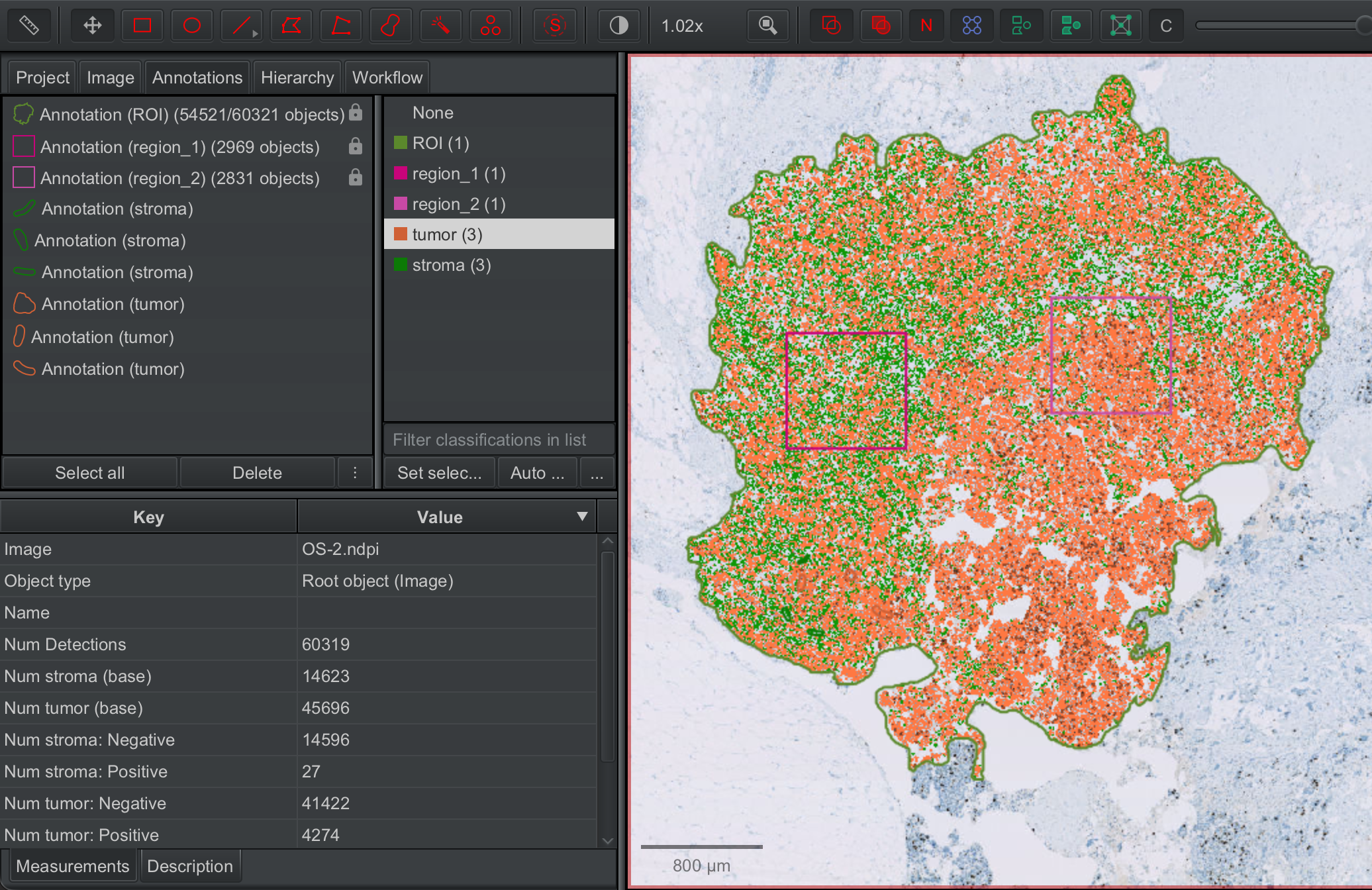
8. The cells detected within ROI will therefore be either of the following four classes:

• tumor: positive (brown outline)

• tumor: negative (orange outline)

• stroma: positive (dark green outline)

• stroma: negative (light green outline) In addition, we will also known whether the cells were present in region_1, region_2, or outside these regions.

In addition to the classification, we will also know whether the cell was present in region_1, region_2, or outside these regions.

2.2.6 View and export detection measurements

---

Measure additional features

QuPath measures some size/shape and intensity features for all the annotations and detections by default. However, you can also obtain more granular or more advanced measurements that take into consideration more contextual information. To do this, you can click on Analyze --> Calculate features and then select the features that you would want to extract.

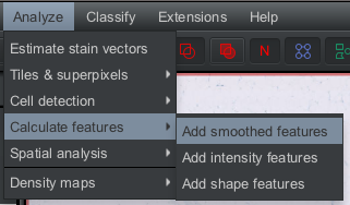
For the type of image we are analyzing, you may want to compute these additional intensity features.

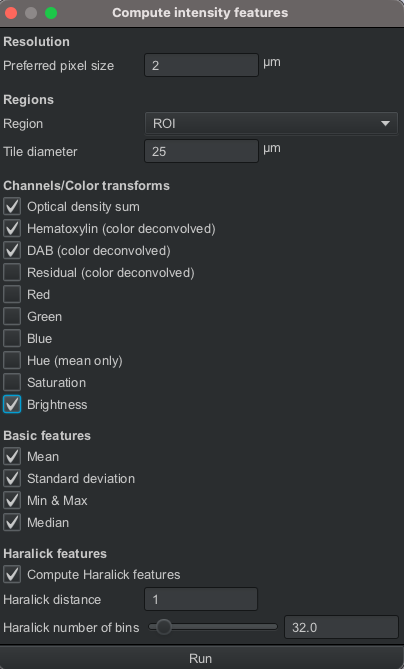
We would want these measurements for all Detections

View detection measurements

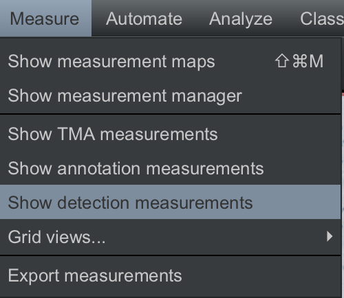
• Detection measurements can be viewed by clicking Measure --> Show detection measurements

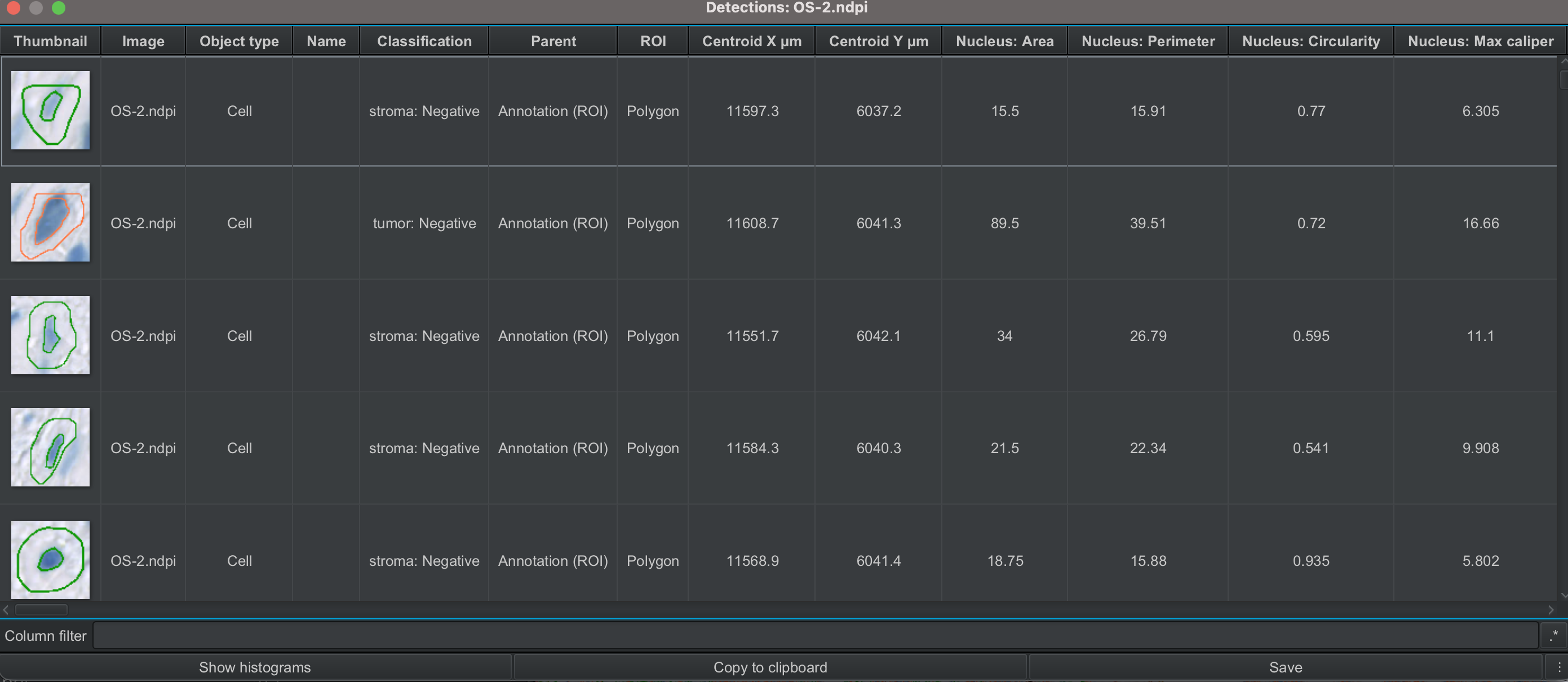
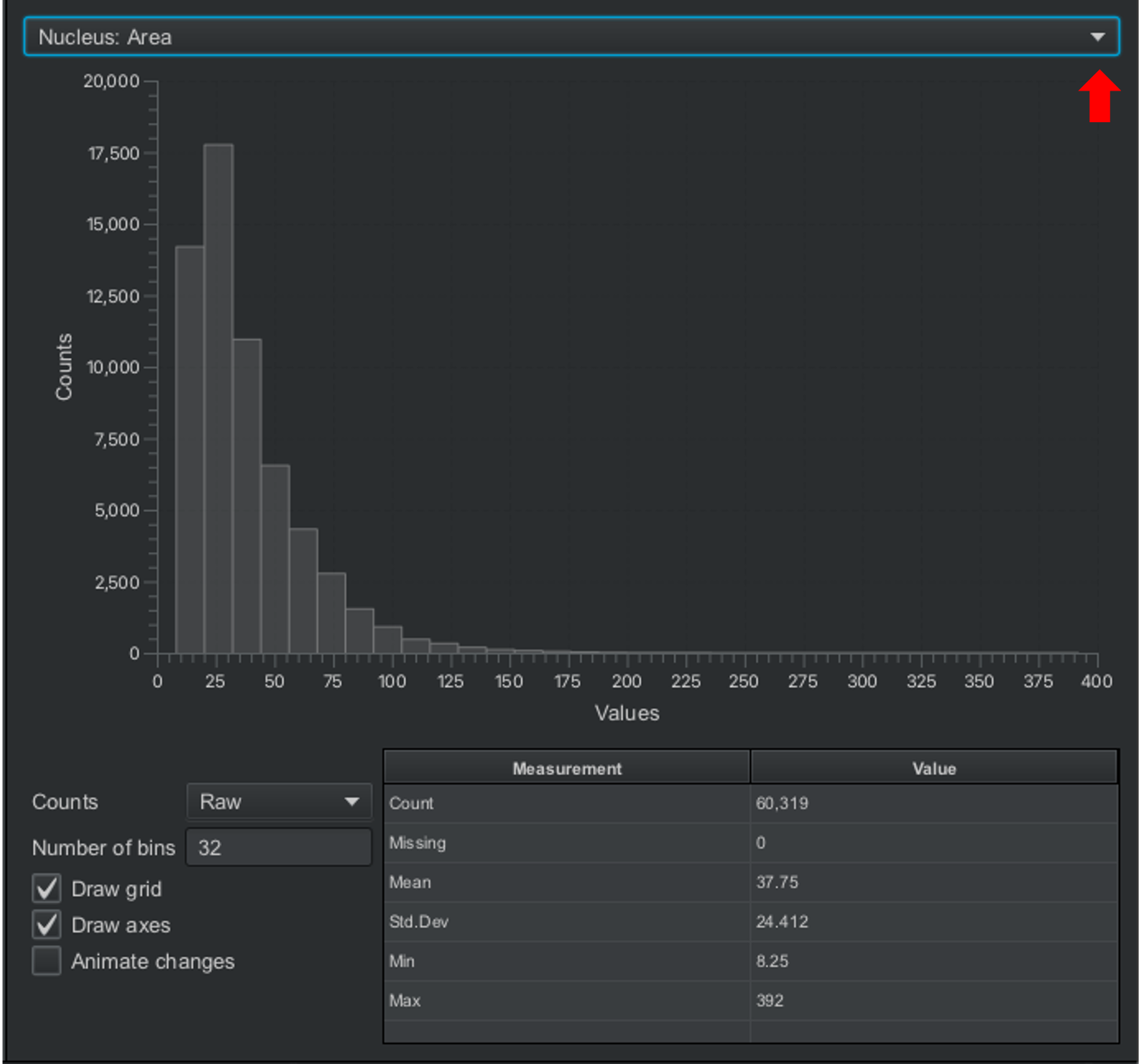
You can click Show histograms to visualize the distribution of cell counts for each metric. To choose a specific metric, use the dropdown menu (red arrow).

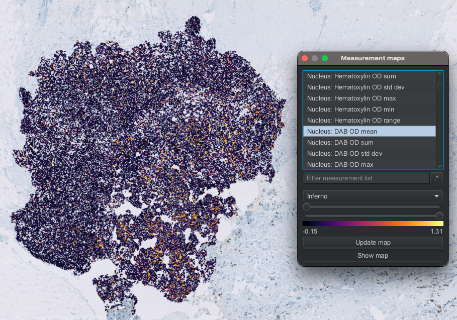
• You can also visualize the measurements as a heatmap overlaid on the image by clicking Measure --> Show measurement maps. You can choose the measurement you want to display and the color map, and also adjust how the color is displayed with the sliders. Here, I have displayed Nucleus: DAB OD Mean using the color map Inferno.

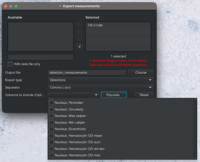
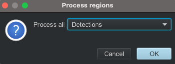
• Finally, to export the measurements, you can click on Measure --> Export measurements and select the objects for which you want to export the measurements (e.g. annotations, detections). We will name the file, select Detections and set the separator to .csv.

You will see the file with single-cell data saved in your QuPath project folder!

⚠️ Hint: The step above will export all the measurements. However, if you are interested in exporting only a specific subset of the measurements, click Populate and check the boxes of the measurements that you want to export!

---

---

Congrats! 🎉 You have now learned the basics of QuPath! ✨

---