18 DIY Lab
library(Seurat)
library(dplyr)
library(Matrix)
library(gdata)
library(utils)
library(liger)
library(SingleCellExperiment)
library(destiny)
library(scater)
library(clusterExperiment)
library(gam)
library(corrplot)
library(ggplot2)
library(ggthemes)
library(ggbeeswarm)
library(cowplot)
library(RColorBrewer)
18.1 DIY Lab
Hopefully now you have a “feel” for what scRNA-seq analysis entails. Today we will work in groups to analyze a publicly available data set: IDH-mutated gliomas. Your data includes: IDH_A_processed_data_portal.txt - the TPM matrix, already in log scale IDH_A_cell_type_assignment_portal.txt - a classification of cells to malignant and non-malignant groups, and to tumors You also have files for different signatures.
What would you like to focus on today? If it’s clustering and identifying cell populations we reccomend you use all the data and try to distinguish the different cell types. If it’s combining a few datasets and work on batch correction, we reccomend you focus on all malignant cells and work on the batch effects among tumors and identifying cell populations shared among them. If it’s identifying subtle differenced in clustering and trying also to identify lineages we reccomend you use one tumor. Most importantly, feel free to explore what ever interest you!
# read the single cell RNA data
sc.data.dirname <- "data/lab20_DIY/"

# if your rstudio crashes and you would like to use a smaller dataset
counts <- read.table(file = paste0(sc.data.dirname,"/IDH_A_processed_data_portal_filtered.txt"), sep="\t", header = TRUE, row.names=1)
classification <- read.table(file = paste0(sc.data.dirname,"/IDH_A_cell_type_assignment_portal_filtered.txt"), sep="\t", header = TRUE)
Create a seurat object filtering out the very extreme cases.
## Warning: Feature names cannot have underscores ('_'), replacing with dashes
## ('-')
vec.cell.type <- classification$type
names(vec.cell.type) <- classification$cell_name
seurat <- AddMetaData(object = seurat, metadata = vec.cell.type, col.name = "cell_type")
vec.tumor.name <- classification$tumor_name
names(vec.tumor.name) <- classification$cell_name
seurat <- AddMetaData(object = seurat, metadata = vec.tumor.name, col.name = "tumor_name")#Notice: Unfortunetlay this dataset does not provide mitochondrial genes so we cannot calculate percent.mito
# load resources
resources.dirname <- "data/resources/"
# Load the the list of house keeping genes
hkgenes <- read.table(paste0(resources.dirname,"/tirosh_house_keeping.txt"), skip = 2)
hkgenes <- as.vector(hkgenes$V1)
# remove hkgenes that were not found
hkgenes.found <- which(toupper(rownames(seurat@assays$RNA)) %in% hkgenes)
n.expressed.hkgenes <- Matrix::colSums(seurat@assays$RNA[hkgenes.found, ] > 0)
seurat <- AddMetaData(object = seurat, metadata = n.expressed.hkgenes, col.name = "n.exp.hkgenes")
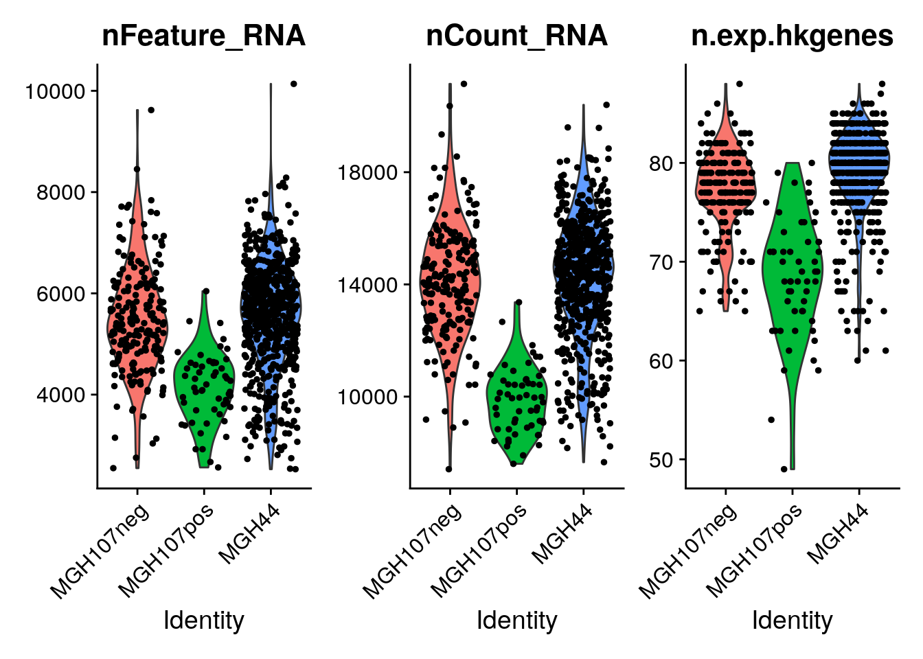
VlnPlot(object = seurat, features = c("nFeature_RNA", "nCount_RNA","n.exp.hkgenes"), ncol = 3)
You can start by filtering extreme outliers if you would like (just replace the ‘?’)
And normalize:
# Read in a list of cell cycle markers, from Tirosh et al, 2015.
# We can segregate this list into markers of G2/M phase and markers of S phase.
s.genes <- Seurat::cc.genes$s.genes
g2m.genes <- Seurat::cc.genes$g2m.genes
seurat <- CellCycleScoring(object = seurat, s.features = s.genes, g2m.features = g2m.genes, set.ident = TRUE)
seurat <- AddModuleScore(object = seurat, features = list(read.table(paste0(resources.dirname,"astro_genes.txt"))$V1), name = "astro_signature")
seurat <- AddModuleScore(object = seurat, features = list(read.table(paste0(resources.dirname,"oligo_genes.txt"))$V1), name = "oligo_signature")
seurat <- AddModuleScore(object = seurat, features = list(read.table(paste0(resources.dirname,"stemness_genes.txt"))$V1), name = "stemness_signature")NOTICE: THESE FOLLOWING COMMANDS WILL ONLY WORK AFTER CREATEING UMAP/tSNE Here are useful markers that can be used to explore the clusters after you will cluster the data
FeaturePlot(seurat, features = c("CD14","CSF1R","FCER1G","FCGR3A")) # markers for macrophages
FeaturePlot(seurat, features = c("MBP","MAG","MOG")) # markers for oligodendrocytes
And a few useful commands, that can be used after clustering:
# notice that the name of the signature is the name you assigned to it, plus "1" that seurat is adding to it
FeaturePlot(seurat, features = c("oligo_signature1","astro_signature1","stemness_signature1"))
If you want to focus on just malignant cells, or just one tumor at a time
seurat.malignant<- subset(seurat, subset = cell_type == "malignant") #keep only malignant cells
seurat.malignant.MGH107<- subset(seurat.malignant, subset = tumor_name == "MGH107neg") #keep only malignant MGH107 cells
seurat.malignant.MGH44<- subset(seurat.malignant, subset = tumor_name == "MGH44") #keep only malignant MGH44 cells
Ok, you are ready! Discuss what you wish to explore and go for it!