12 Batch Correction Lab
In this lab, we will look at different single cell RNA-seq datasets collected from pancreatic islets. We will look at how different batch correction methods affect our data analysis.
Note: you can increase the system memory available to Docker by going to Docker -> Preferences -> Advanced and shifting the Memory slider.
12.1 Load settings and packages
## Loading required package: sp## Loading required package: maps## Loading required package: shapefiles## Loading required package: foreign##
## Attaching package: 'shapefiles'## The following objects are masked from 'package:foreign':
##
## read.dbf, write.dbf## ------------------------------------------------------------------------------## You have loaded plyr after dplyr - this is likely to cause problems.
## If you need functions from both plyr and dplyr, please load plyr first, then dplyr:
## library(plyr); library(dplyr)## ------------------------------------------------------------------------------##
## Attaching package: 'plyr'## The following object is masked from 'package:maps':
##
## ozone## The following objects are masked from 'package:dplyr':
##
## arrange, count, desc, failwith, id, mutate, rename, summarise,
## summarize## Loading required package: cowplot##
## ********************************************************## Note: As of version 1.0.0, cowplot does not change the## default ggplot2 theme anymore. To recover the previous## behavior, execute:
## theme_set(theme_cowplot())## ********************************************************## Loading required package: patchwork##
## Attaching package: 'patchwork'## The following object is masked from 'package:cowplot':
##
## align_plots# Set folder location for saving output files. This is also the same location as input data.
mydir <- "data/batch_correction/"
setwd("/home/rstudio/materials/")
# Objects to save.
Rda.sparse.path <- paste0(mydir, "pancreas_subsample.Rda")
Rda.path <- paste0(mydir, "pancreas_nobatchcorrect.Rda")
Rda.Seurat3.path <- paste0(mydir, "pancreas_Seurat3.Rda")
Rda.liger.path <- paste0(mydir, "pancreas_liger.Rda")12.2 Read in pancreas expression matrices
# Read in all four input expression matrices
celseq.data <- read.table(paste0(mydir, "pancreas_multi_celseq_expression_matrix.txt.gz"))
celseq2.data <- read.table(paste0(mydir, "pancreas_multi_celseq2_expression_matrix.txt.gz"))
fluidigmc1.data <- read.table(paste0(mydir, "pancreas_multi_fluidigmc1_expression_matrix.txt.gz"))
smartseq2.data <- read.table(paste0(mydir, "pancreas_multi_smartseq2_expression_matrix.txt.gz"))

# Convert to sparse matrices for efficiency
celseq.data <- as(as.matrix(celseq.data), "dgCMatrix")
celseq2.data <- as(as.matrix(celseq2.data), "dgCMatrix")
fluidigmc1.data <- as(as.matrix(fluidigmc1.data), "dgCMatrix")
smartseq2.data <- as(as.matrix(smartseq2.data), "dgCMatrix")
12.3 Preparing the individual Seurat objects for each pancreas dataset without batch correction
# What is the size of each single cell RNA-seq dataset?
# Briefly describe the technology used to collect each dataset.
# Which datasets do you expect to be different and which do you expect to be similar?
dim(celseq.data)
dim(celseq2.data)
dim(fluidigmc1.data)
dim(smartseq2.data)

# Create and setup Seurat objects for each dataset with the following 6 steps.
# 1. CreateSeuratObject
# 2. subset
# 3. NormalizeData
# 4. FindVariableFeatures
# 5. ScaleData
# 6. Update @meta.data slot in Seurat object with tech column (celseq, celseq2, fluidigmc1, smartseq2)
# Look at the distributions of number of genes per cell before and after FilterCells.

# CEL-Seq (https://www.cell.com/cell-reports/fulltext/S2211-1247(12)00228-8)
# In subset, use low.thresholds = 1750
celseq <- CreateSeuratObject(counts = celseq.data)
VlnPlot(celseq, "nFeature_RNA")
celseq <- subset(celseq, subset = nFeature_RNA > 1750)
VlnPlot(celseq, "nFeature_RNA")
celseq <- NormalizeData(celseq, normalization.method = "LogNormalize", scale.factor = 10000)
celseq <- FindVariableFeatures(celseq, selection.method = "vst", nfeatures = 2000)
celseq <- ScaleData(celseq)
celseq[["tech"]] <- "celseq"

# CEL-Seq2 https://www.cell.com/molecular-cell/fulltext/S1097-2765(09)00641-8
# In subset, use low.thresholds = 2500.
celseq2 <- CreateSeuratObject(counts = celseq2.data)
VlnPlot(celseq2, "nFeature_RNA")
celseq2 <- subset(celseq2, subset = nFeature_RNA > 2500)
VlnPlot(celseq2, "nFeature_RNA")
celseq2 <- NormalizeData(celseq2, normalization.method = "LogNormalize", scale.factor = 10000)
celseq2 <- FindVariableFeatures(celseq2, selection.method = "vst", nfeatures = 2000)
celseq2 <- ScaleData(celseq2)
celseq2[["tech"]] <- "celseq2"

# Fluidigm C1
# Omit subset function because cells are already high quality.
fluidigmc1 <- CreateSeuratObject(counts = fluidigmc1.data)
VlnPlot(fluidigmc1, "nFeature_RNA")
fluidigmc1 <- NormalizeData(fluidigmc1, normalization.method = "LogNormalize", scale.factor = 10000)
fluidigmc1 <- FindVariableFeatures(fluidigmc1, selection.method = "vst", nfeatures = 2000)
fluidigmc1 <- ScaleData(fluidigmc1)
fluidigmc1[["tech"]] <- "fluidigmc1"

# SMART-Seq2
# In subset, use low.thresholds = 2500.
smartseq2 <- CreateSeuratObject(counts = smartseq2.data)
VlnPlot(smartseq2, "nFeature_RNA")
smartseq2 <- subset(smartseq2, subset = nFeature_RNA > 2500)
VlnPlot(smartseq2, "nFeature_RNA")
smartseq2 <- NormalizeData(smartseq2, normalization.method = "LogNormalize", scale.factor = 10000)
smartseq2 <- FindVariableFeatures(smartseq2, selection.method = "vst", nfeatures = 2000)
smartseq2 <- ScaleData(smartseq2)
smartseq2[["tech"]] <- "smartseq2"

# This code sub-samples the data in order to speed up calculations and not use too much memory.
Idents(celseq) <- "tech"
celseq <- subset(celseq, downsample = 500, seed = 1)
Idents(celseq2) <- "tech"
celseq2 <- subset(celseq2, downsample = 500, seed = 1)
Idents(fluidigmc1) <- "tech"
fluidigmc1 <- subset(fluidigmc1, downsample = 500, seed = 1)
Idents(smartseq2) <- "tech"
smartseq2 <- subset(smartseq2, downsample = 500, seed = 1)

# Save the sub-sampled Seurat objects
save(celseq, celseq2, fluidigmc1, smartseq2, file = Rda.sparse.path)
12.4 Cluster pancreatic datasets without batch correction
Let us cluster all the pancreatic islet datasets together and see whether there is a batch effect.
load(Rda.sparse.path)

# Merge Seurat objects. Original sample identities are stored in gcdata[["tech"]].
# Cell names will now have the format tech_cellID (smartseq2_cell1...)
add.cell.ids <- c("celseq", "celseq2", "fluidigmc1", "smartseq2")
gcdata <- merge(x = celseq, y = list(celseq2, fluidigmc1, smartseq2), add.cell.ids = add.cell.ids, merge.data = FALSE)
Idents(gcdata) <- "tech"  # use identity based on sample identity

# Look at how the number of genes per cell varies across the different technologies.
VlnPlot(gcdata, "nFeature_RNA", group.by = "tech")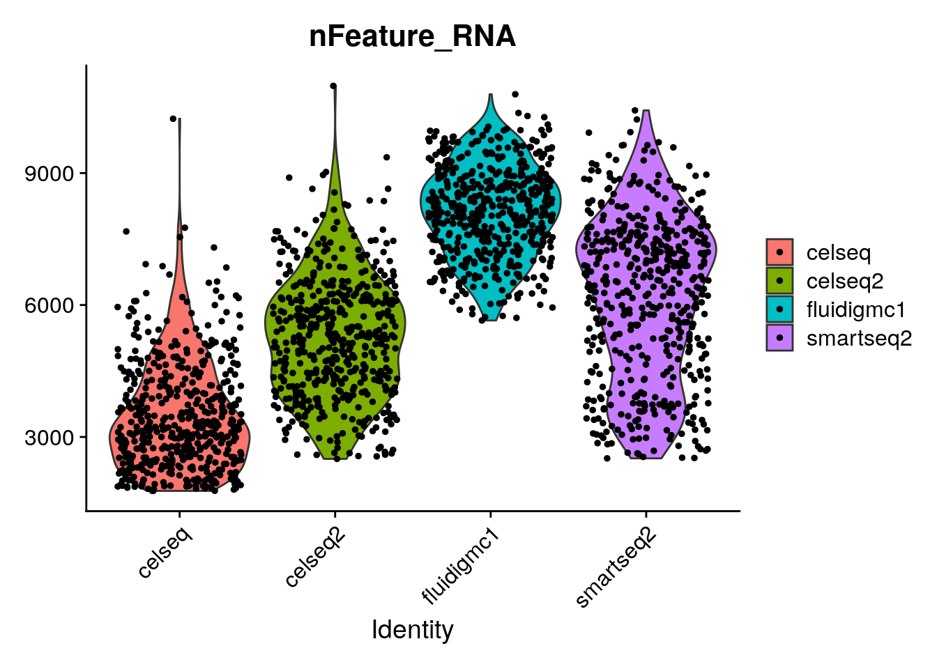
# The merged data must be normalized and scaled (but you only need to scale the variable genes).
# Let us also find the variable genes again this time using all the pancreas data.
gcdata <- NormalizeData(gcdata, normalization.method = "LogNormalize", scale.factor = 10000)
var.genes <- SelectIntegrationFeatures(SplitObject(gcdata, split.by = "tech"), nfeatures = 2000, verbose = TRUE, fvf.nfeatures = 2000, selection.method = "vst")
## No variable features found for object1 in the object.list. Running FindVariableFeatures ...## No variable features found for object2 in the object.list. Running FindVariableFeatures ...## No variable features found for object3 in the object.list. Running FindVariableFeatures ...## No variable features found for object4 in the object.list. Running FindVariableFeatures ...VariableFeatures(gcdata) <- var.genes
gcdata <- ScaleData(gcdata, features = VariableFeatures(gcdata))## Centering and scaling data matrix# Do PCA on data including only the variable genes.
gcdata <- RunPCA(gcdata, features = VariableFeatures(gcdata), npcs = 40, ndims.print = 1:5, nfeatures.print = 5)## PC_ 1
## Positive: CHGB, SCG2, PAM, ABCC8, MIR7-3HG
## Negative: IFITM3, ZFP36L1, TACSTD2, LGALS3, ANXA4
## PC_ 2
## Positive: COL1A2, SPARC, COL5A1, COL3A1, SFRP2
## Negative: ELF3, KRT8, CD24, ATP1B1, SERPINA3
## PC_ 3
## Positive: HIF1A, CTSD, ITGB6, PEMT, DHRS3
## Negative: LOC100131257, PGM5P2, UGDH-AS1, MAB21L3, LOC643406
## PC_ 4
## Positive: CPA2, CTRC, CTRB2, PLA2G1B, CTRB1
## Negative: CFTR, VTCN1, AQP1, TINAGL1, ALDH1A3
## PC_ 5
## Positive: GC, TM4SF4, IRX2, TMEM176A, ARX
## Negative: PFKFB2, HADH, INS, IAPP, ADCYAP1# Color the PC biplot by the scRNA-seq technology. Hint: use DimPlot
# Which technologies look similar to one another?
DimPlot(gcdata, reduction = "pca", dims = c(1, 2), group.by = "tech")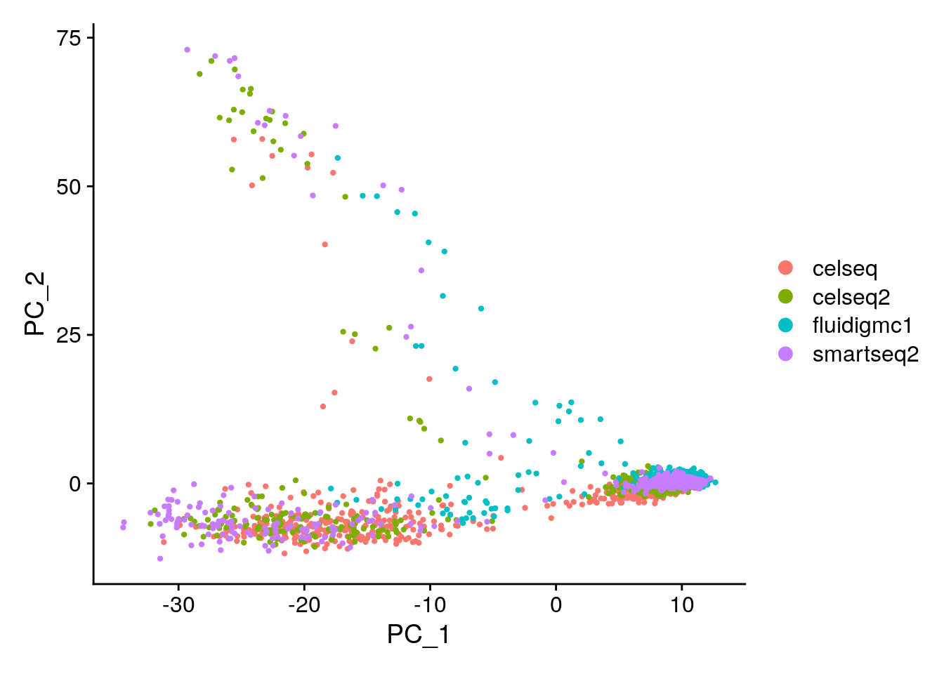
# Cluster the cells using the first twenty principal components.
gcdata <- FindNeighbors(gcdata, reduction = "pca", dims = 1:20, k.param = 20)
## Computing nearest neighbor graph## Computing SNN## Modularity Optimizer version 1.3.0 by Ludo Waltman and Nees Jan van Eck
##
## Number of nodes: 2000
## Number of edges: 60309
##
## Running Louvain algorithm...
## Maximum modularity in 10 random starts: 0.9169
## Number of communities: 17
## Elapsed time: 0 seconds# Create a UMAP visualization.
gcdata <- RunUMAP(gcdata, dims = 1:20, reduction = "pca", n.neighbors = 15, min.dist = 0.5, spread = 1, metric = "euclidean", seed.use = 1) ## Warning: The default method for RunUMAP has changed from calling Python UMAP via reticulate to the R-native UWOT using the cosine metric
## To use Python UMAP via reticulate, set umap.method to 'umap-learn' and metric to 'correlation'
## This message will be shown once per session## 19:58:49 UMAP embedding parameters a = 0.583 b = 1.334## 19:58:49 Read 2000 rows and found 20 numeric columns## 19:58:49 Using FNN for neighbor search, n_neighbors = 15## 19:58:49 Commencing smooth kNN distance calibration using 1 thread## 19:58:50 Initializing from normalized Laplacian + noise## 19:58:50 Commencing optimization for 500 epochs, with 39212 positive edges## 19:58:52 Optimization finished# Visualize the Louvain clustering and the batches on the UMAP.
# Remember, the clustering is stored in @meta.data in column seurat_clusters and the technology is
# stored in the column tech. Remember you can also use DimPlot
DimPlot(gcdata, reduction = "umap", group.by = "seurat_clusters")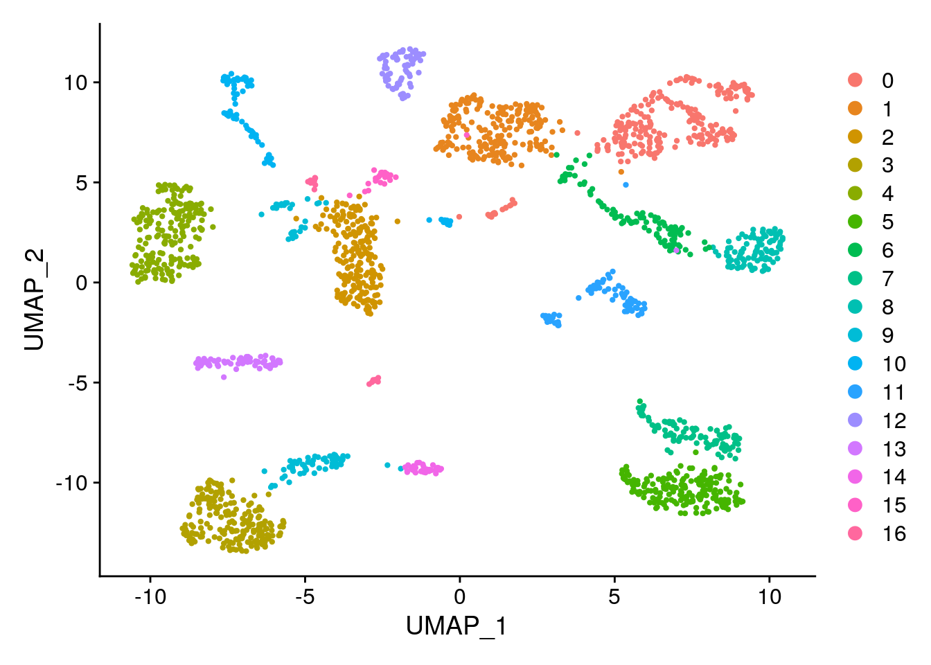
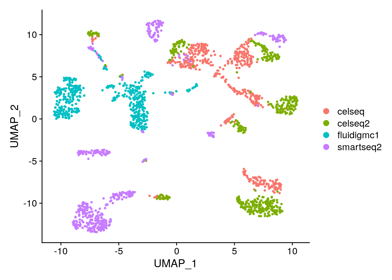
# Are you surprised by the results? Compare to your expectations from the PC biplot of PC1 vs PC2.
# What explains these results?

# Adjusted rand index test for overlap between technology and cluster labelings.
# This goes between 0 (completely dissimilar clustering) to 1 (identical clustering).
# The adjustment corrects for chance grouping between cluster elements.
# https://davetang.org/muse/2017/09/21/adjusted-rand-index/
ari <- dplyr::select(gcdata[[]], tech, seurat_clusters)
ari$tech <- plyr::mapvalues(ari$tech, from = c("celseq", "celseq2", "fluidigmc1", "smartseq2"), to = c(0, 1, 2, 3))
adj.rand.index(as.numeric(ari$tech), as.numeric(ari$seurat_clusters))
## [1] 0.7817657# Save current progress.
save(gcdata, file = Rda.path)
# To load the data, run the following command.
# load(Rda.path)12.4.1 Batch correction: canonical correlation analysis (CCA) + mutual nearest neighbors (MNN) using Seurat v3
Here we use Seurat v3 to see to what extent it can remove potential batch effects.
# load(Rda.sparse.path)

# The first piece of code will identify variable genes that are highly variable in at least 2/4 datasets. We will use these variable genes in our batch correction.
# Why would we implement such a requirement?
ob.list <- list(celseq, celseq2, fluidigmc1, smartseq2)

# Identify anchors on the 4 pancreatic islet datasets, commonly shared variable genes across samples,
# and integrate samples.
gcdata.anchors <- FindIntegrationAnchors(object.list = ob.list, anchor.features = 2000, dims = 1:30)
## Computing 2000 integration features## Scaling features for provided objects## Finding all pairwise anchors## Running CCA## Merging objects## Finding neighborhoods## Finding anchors## Found 1569 anchors## Filtering anchors## Retained 1486 anchors## Extracting within-dataset neighbors## Running CCA## Merging objects## Finding neighborhoods## Finding anchors## Found 1481 anchors## Filtering anchors## Retained 1273 anchors## Extracting within-dataset neighbors## Running CCA## Merging objects## Finding neighborhoods## Finding anchors## Found 1621 anchors## Filtering anchors## Retained 1450 anchors## Extracting within-dataset neighbors## Running CCA## Merging objects## Finding neighborhoods## Finding anchors## Found 1554 anchors## Filtering anchors## Retained 1413 anchors## Extracting within-dataset neighbors## Running CCA## Merging objects## Finding neighborhoods## Finding anchors## Found 1693 anchors## Filtering anchors## Retained 1618 anchors## Extracting within-dataset neighbors## Running CCA## Merging objects## Finding neighborhoods## Finding anchors## Found 1576 anchors## Filtering anchors## Retained 1433 anchors## Extracting within-dataset neighbors## Merging dataset 4 into 2## Extracting anchors for merged samples## Finding integration vectors## Finding integration vector weights## Integrating data## Merging dataset 3 into 2 4## Extracting anchors for merged samples## Finding integration vectors## Finding integration vector weights## Integrating data## Merging dataset 1 into 2 4 3## Extracting anchors for merged samples## Finding integration vectors## Finding integration vector weights## Integrating data## Warning: Adding a command log without an assay associated with itDefaultAssay(gcdata) <- "integrated"
# Run the standard workflow for visualization and clustering.
# The integrated data object only stores the commonly shared variable genes.
gcdata <- ScaleData(gcdata, do.center = T, do.scale = F)## Centering data matrix## PC_ 1
## Positive: CHGB, CHGA, VGF, ABCC8, G6PC2
## Negative: REG1A, SERPINA3, REG1B, SPINK1, TACSTD2
## PC_ 2
## Positive: REG1B, REG1A, CTRB2, PRSS1, SPINK1
## Negative: IGFBP7, CFTR, SPP1, PMEPA1, ANXA2
## PC_ 3
## Positive: INS, IAPP, RBP4, PCSK1, HADH
## Negative: TM4SF4, GC, KCTD12, CHGB, RGS4
## PC_ 4
## Positive: SPP1, CFTR, ANXA4, ONECUT2, SLC4A4
## Negative: SPARC, COL1A1, COL1A2, COL3A1, FN1
## PC_ 5
## Positive: INS, G6PC2, VGF, GC, LOXL4
## Negative: PPY, AQP3, SST, ID2, ETV1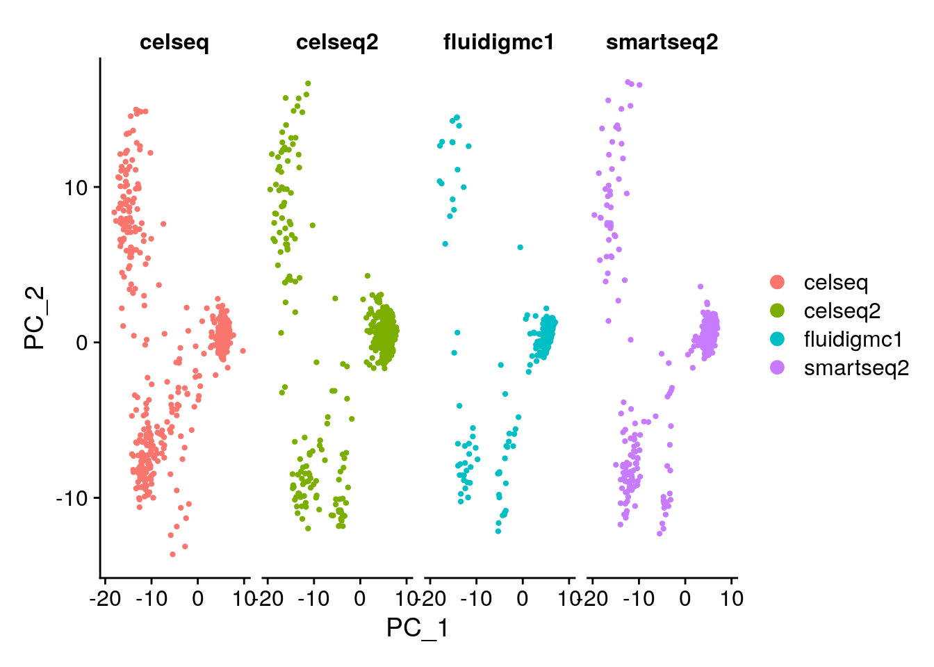
# Clustering. Choose the dimensional reduction type to use and the number of aligned
# canonical correlation vectors to use.
gcdata <- FindNeighbors(gcdata, reduction = "pca", dims = 1:20, k.param = 20)
## Computing nearest neighbor graph## Computing SNN## Modularity Optimizer version 1.3.0 by Ludo Waltman and Nees Jan van Eck
##
## Number of nodes: 2000
## Number of edges: 82031
##
## Running Louvain algorithm...
## Maximum modularity in 10 random starts: 0.8403
## Number of communities: 9
## Elapsed time: 0 seconds# UMAP. Choose the dimensional reduction type to use and the number of aligned
# canonical correlation vectors to use.
gcdata <- RunUMAP(gcdata, dims = 1:30, reduction = "pca", n.neighbors = 15, min.dist = 0.5, spread = 1, metric = "euclidean", seed.use = 1) ## 19:59:41 UMAP embedding parameters a = 0.583 b = 1.334## 19:59:41 Read 2000 rows and found 30 numeric columns## 19:59:41 Using FNN for neighbor search, n_neighbors = 15## 19:59:42 Commencing smooth kNN distance calibration using 1 thread## 19:59:42 Initializing from normalized Laplacian + noise## 19:59:42 Commencing optimization for 500 epochs, with 44578 positive edges## 19:59:44 Optimization finished# After data integration, use the original expression data in all visualization and DE tests.
# The integrated data must not be used in DE tests as it violates assumptions of independence in DE tests!
DefaultAssay(gcdata) <- "RNA"
# Visualize the Louvain clustering and the batches on the UMAP.
# Remember, the clustering is stored in @meta.data in column seurat_clusters
# and the technology is stored in the column tech. Remember you can also use DimPlot.
p1 <- DimPlot(gcdata, reduction = "umap", group.by = "seurat_clusters")
p2 <- DimPlot(gcdata, reduction = "umap", group.by = "tech")
p1 + p2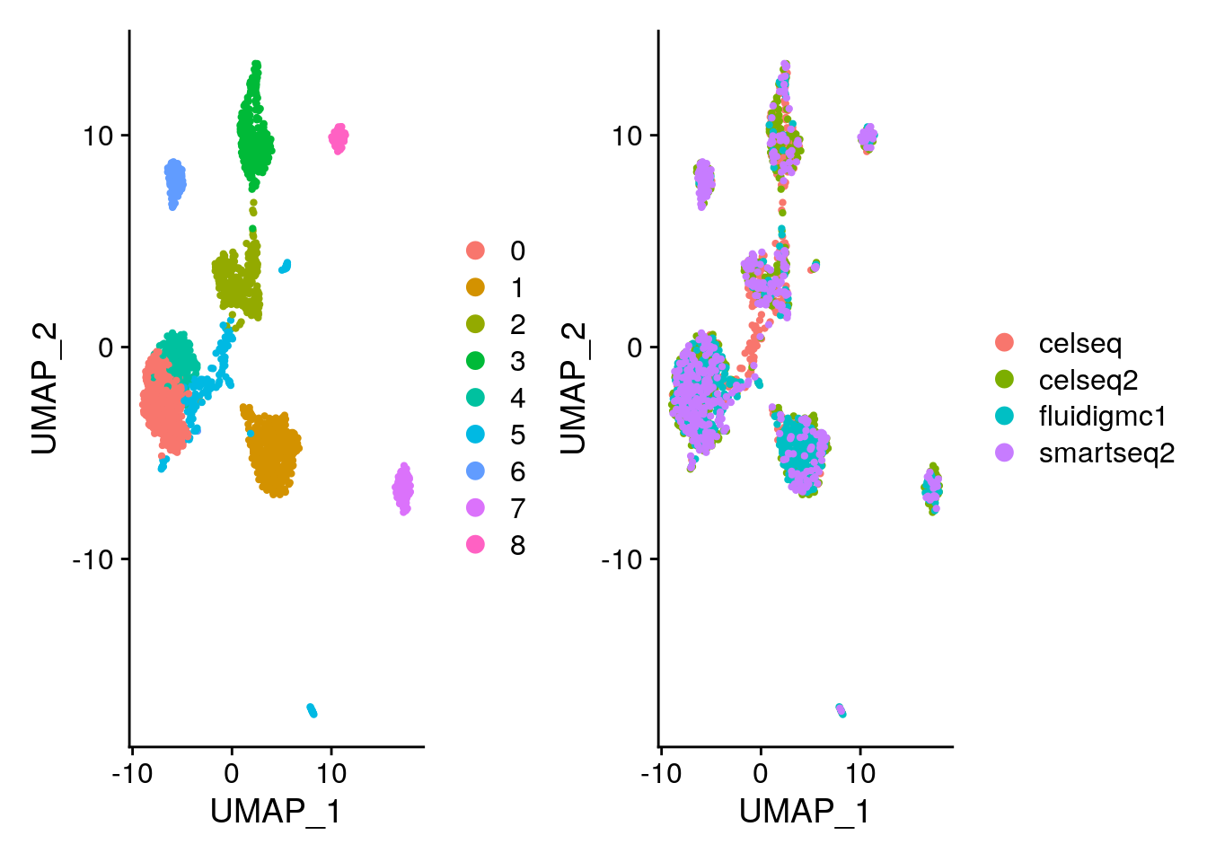
# Let's look to see how the adjusted rand index changed compared to using no batch correction.
ari <- dplyr::select(gcdata[[]], tech, seurat_clusters)
ari$tech <- plyr::mapvalues(ari$tech, from = c("celseq", "celseq2", "fluidigmc1", "smartseq2"), to = c(0, 1, 2, 3))
adj.rand.index(as.numeric(ari$tech), as.numeric(ari$seurat_clusters))
## [1] 0.2910816# We can also identify conserved marker genes across the batches. Differential gene expression is
# done across each batch, and the p-values are combined.
markers <- FindConservedMarkers(gcdata, ident.1 = 0, grouping.var = "tech", assay = "RNA", print.bar = T)## Testing group celseq: (0) vs (2, 5, 3, 1, 7, 8, 4, 6)## Testing group celseq2: (0) vs (2, 7, 3, 4, 5, 6, 1, 8)## Testing group fluidigmc1: (0) vs (1, 2, 5, 3, 4, 6, 8, 7)## Testing group smartseq2: (0) vs (6, 5, 3, 1, 7, 4, 2, 8)## celseq_p_val celseq_avg_logFC celseq_pct.1 celseq_pct.2 celseq_p_val_adj
## TTR 3.390774e-38 2.484763 1.000 0.840 1.140419e-33
## IRX2 5.412444e-55 1.444636 0.914 0.114 1.820367e-50
## GC 6.002464e-45 1.735058 0.971 0.223 2.018809e-40
## TM4SF4 1.689266e-40 2.077775 1.000 0.447 5.681508e-36
## PCSK2 9.449515e-39 1.967239 1.000 0.502 3.178155e-34
## CRYBA2 1.219002e-45 2.175575 0.986 0.249 4.099868e-41
## celseq2_p_val celseq2_avg_logFC celseq2_pct.1 celseq2_pct.2
## TTR 1.739228e-48 1.616678 1.000 1.000
## IRX2 1.986638e-45 1.039948 0.982 0.296
## GC 2.408920e-41 1.464222 0.991 0.637
## TM4SF4 6.084562e-42 1.428749 1.000 0.675
## PCSK2 3.067042e-41 1.205282 1.000 0.930
## CRYBA2 5.114040e-44 1.342788 0.964 0.312
## celseq2_p_val_adj fluidigmc1_p_val fluidigmc1_avg_logFC fluidigmc1_pct.1
## TTR 5.849545e-44 1.309385e-47 1.5276204 1.000
## IRX2 6.681658e-41 5.587069e-40 0.3931639 0.871
## GC 8.101920e-37 8.305073e-52 1.3483970 0.992
## TM4SF4 2.046421e-37 2.281765e-51 1.6572137 1.000
## PCSK2 1.031538e-36 1.610934e-29 0.8852347 1.000
## CRYBA2 1.720005e-39 3.177304e-30 0.6646222 0.955
## fluidigmc1_pct.2 fluidigmc1_p_val_adj smartseq2_p_val
## TTR 0.932 4.403854e-43 2.285127e-56
## IRX2 0.204 1.879099e-35 1.192243e-47
## GC 0.288 2.793245e-47 1.422158e-38
## TM4SF4 0.443 7.674259e-47 3.349777e-42
## PCSK2 0.870 5.418054e-25 6.430694e-51
## CRYBA2 0.473 1.068623e-25 9.436894e-50
## smartseq2_avg_logFC smartseq2_pct.1 smartseq2_pct.2 smartseq2_p_val_adj
## TTR 1.7368710 1.000 1.000 7.685568e-52
## IRX2 0.7954382 0.894 0.235 4.009871e-43
## GC 1.1002339 1.000 0.685 4.783145e-34
## TM4SF4 1.2984975 1.000 0.822 1.126630e-37
## PCSK2 1.3372298 1.000 0.716 2.162835e-46
## CRYBA2 1.8649270 1.000 0.630 3.173910e-45
## max_pval minimump_p_val
## TTR 3.390774e-38 9.140508e-56
## IRX2 5.587069e-40 2.164978e-54
## GC 1.422158e-38 3.322029e-51
## TM4SF4 1.689266e-40 9.127059e-51
## PCSK2 1.610934e-29 2.572278e-50
## CRYBA2 3.177304e-30 3.774757e-49# Visualize the expression of the first 5 marker genes on UMAP across the different batches using DoHeatmap.
gcdata <- ScaleData(gcdata, features = rownames(gcdata), do.center = T, do.scale = F)## Centering data matrix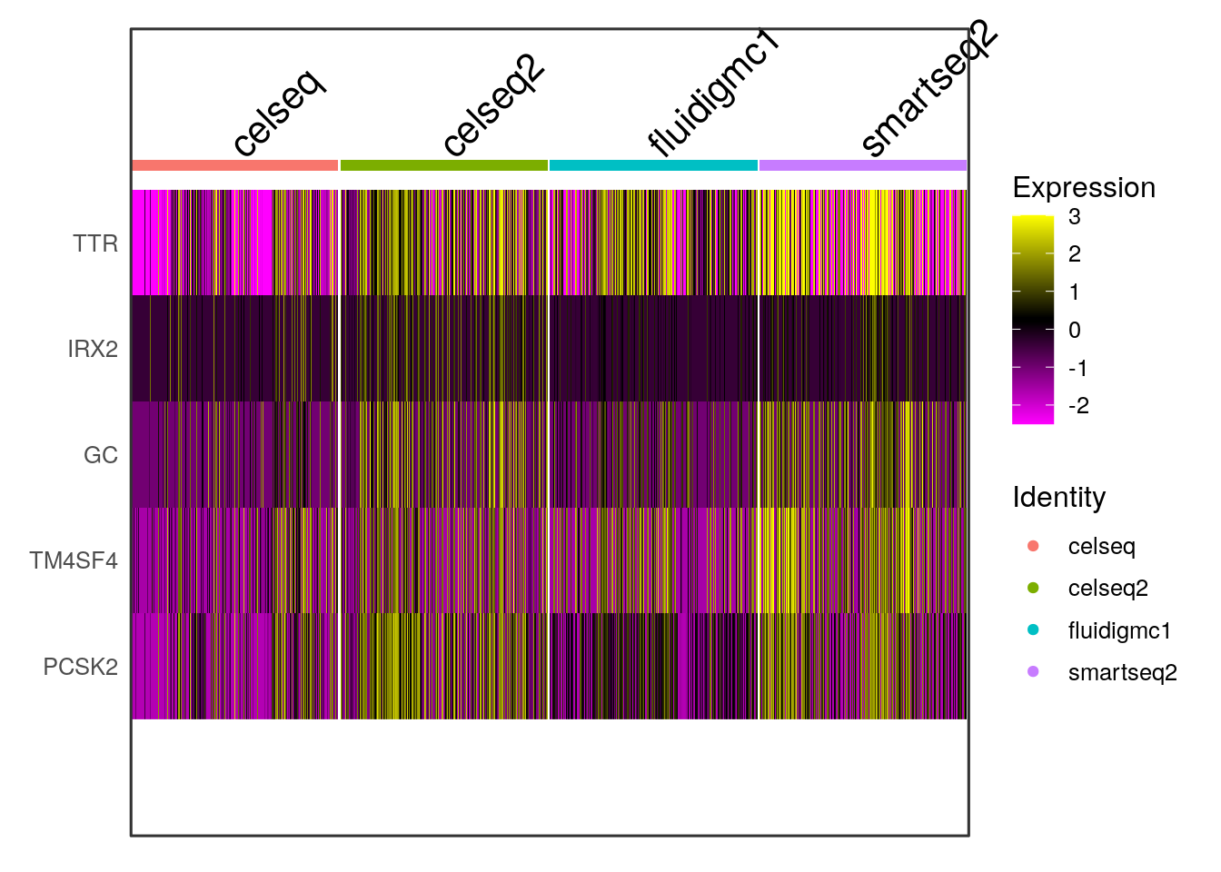
# Markers for pancreatic cells from "A Single-Cell Transcriptome Atlas of the
# Human Pancreas".https://www.cell.com/cell-systems/pdfExtended/S2405-4712(16)30292-7
genes <- c("GCG", "INS", "SST", "PPY", "PRSS1", "KRT19", "PECAM1", "COL1A1")
FeaturePlot(gcdata, genes, ncol = 4)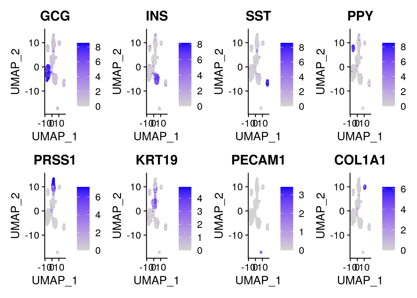
12.4.2 Batch correction: integrative non-negative matrix factorization (NMF) using LIGER
Here we use integrative non-negative matrix factorization to see to what extent it can remove potential batch effects.
The important parameters in the batch correction are the number of factors (k), the penalty parameter (lambda), and the clustering resolution. The number of factors sets the number of factors (consisting of shared and dataset-specific factors) used in factorizing the matrix. The penalty parameter sets the balance between factors shared across the batches and factors specific to the individual batches. The default setting of lambda=5.0 is usually used by the Macosko lab. Resolution=1.0 is used in the Louvain clustering of the shared neighbor factors that have been quantile normalized.
# load(Rda.sparse.path)

ob.list <- list("celseq" = celseq, "celseq2" = celseq2, "fluidigmc1" = fluidigmc1, "smartseq2" = smartseq2)

# Identify variable genes that are variable across most samples.
var.genes <- SelectIntegrationFeatures(ob.list, nfeatures = 2000, verbose = TRUE, fvf.nfeatures = 2000, selection.method = "vst")

# Next we create a LIGER object with raw counts data from each batch.
data.liger <- createLiger(sapply(ob.list, function(data) data[['RNA']]@counts[, colnames(data)]), remove.missing = F)

# Normalize gene expression for each batch.
data.liger <- liger::normalize(data.liger)

# Use my method or Liger method for selecting variable genes (var.thresh changes number of variable genes).
data.liger@var.genes <- var.genes
# data.liger <- selectGenes(data.liger, var.thresh = 0.1, do.plot = F)

# Print out the number of variable genes for LIGER analysis.
print(length(data.liger@var.genes))

# Scale the gene expression across the datasets.
# Why does LIGER not center the data? Hint, think about the use of
# non-negative matrix factorization and the constraints that this imposes.
data.liger <- scaleNotCenter(data.liger)

# These two steps take 10-20 min. Only run them if you finish with the rest of the code.
# Use the `suggestK` function to determine the appropriate number of factors to use.
# Use the `suggestLambda` function to find the smallest lambda for which the alignment metric stabilizes.
# k.suggest <- suggestK(data.liger, k.test = seq(5, 30, 5), plot.log2 = T)
# lambda.suggest <- suggestLambda(gcdata.liger, k.suggest)

# Use alternating least squares (ALS) to factorize the matrix.
# Next, quantile align the factor loadings across the datasets, and do clustering.
k.suggest <- 20  # with this line, we do not use the suggested k by suggestK()
lambda.suggest <- 5  # with this line, we do not use the suggested lambda by suggestLambda()
set.seed(100)  # optimizeALS below is stochastic
data.liger <- optimizeALS(data.liger, k = k.suggest, lamda = lambda.suggest)

# What do matrices H, V, and W represent, and what are their dimensions?
dim(data.liger@H$celseq)
dim(data.liger@V$celseq)
dim(data.liger@W)

# Next, do clustering of cells in shared nearest factor space.
# Build SNF graph, do quantile normalization, cluster quantile normalized data
data.liger <- quantileAlignSNF(data.liger, resolution = 1)  # SNF clustering and quantile alignment

# What are the dimensions of H.norm. What does this represent?
dim(data.liger@H.norm)

# Let's see what the liger data looks like mapped onto a UMAP visualization.
data.liger <- runUMAP(data.liger, n_neighbors = 15, min_dist = 0.5)  # conda install -c conda-forge umap-learn
p <- plotByDatasetAndCluster(data.liger, return.plots = T)
print(p[[1]])  # plot by dataset
plot_grid(p[[1]], p[[2]])

# Let's look to see how the adjusted rand index changed compared to using no batch correction.
tech <- unlist(lapply(1:length(data.liger@H), function(x) {
  rep(names(data.liger@H)[x], nrow(data.liger@H[[x]]))}))
clusters <- data.liger@alignment.clusters
ari <- data.frame("tech" = tech, "clusters" = clusters)
ari$tech <- plyr::mapvalues(ari$tech, from = c("celseq", "celseq2", "fluidigmc1", "smartseq2"), to = c(0, 1, 2, 3))
adj.rand.index(as.numeric(ari$tech), as.numeric(ari$clusters))

# Look at proportion of each batch in each cluster, and look at factor loadings across clusters
plotClusterProportions(data.liger)
plotClusterFactors(data.liger, use.aligned = T)

# Look at genes that are specific to a dataset and shared across datasets.
# Use the plotWordClouds function and choose 2 datasets.
pdf(paste0(mydir, "word_clouds.pdf"))
plotWordClouds(data.liger, dataset1 = "celseq2", dataset2 = "smartseq2")
dev.off()

# Look at factor loadings for each cell using plotFactors.
pdf(paste0(mydir, "plot_factors.pdf"))
plotFactors(data.liger)
dev.off()

# Identify shared and batch-specific marker genes from liger factorization.
# Use the getFactorMarkers function and choose 2 datasets.
# Then plot some genes of interest using plotGene.
markers <- getFactorMarkers(data.liger, dataset1 = "celseq2", dataset2 = "smartseq2", num.genes = 10)
plotGene(data.liger, gene = "INS")

# Save current progress.
save(data.liger, file = Rda.liger.path)
# To load the data, run the following command.
# load(Rda.liger.path)
12.5 Additional exploration: Regressing out unwanted covariates
Learn how to regress out different technical covariates (number of UMIs, number of genes, percent mitochondrial reads) by studying Seurat’s PBMC tutorial and the ScaleData() function.
12.6 Additional exploration: kBET
Within your RStudio session, install k-nearest neighbour batch effect test and learn how to use its functionality to quantify batch effects in the pancreatic data.
12.7 Additional exploration: Seurat 3
Read how new version of Seurat does data integration
12.8 Acknowledgements
This document builds off a tutorial from the Seurat website and a tutorial from the LIGER website.