8 Data Wrangling scRNAseq
8.1 Goal
- To give you experience with the analysis of single cell RNA sequencing (scRNA-seq) including performing quality control and identifying cell type subsets.
- To introduce you to scRNA-seq analysis using the Seurat package.
8.2 Introduction
Data produced in a single cell RNA-seq experiment has several interesting characteristics that make it distinct from data produced in a bulk population RNA-seq experiment. Two characteristics that are important to keep in mind when working with scRNA-Seq are drop-out (the excessive amount of zeros due to limiting mRNA) and the potential for quality control (QC) metrics to be confounded with biology. This combined with the ability to measure heterogeniety from cells in samples has shifted the field away from the typical analysis in population-based RNA-Seq. Here we demonstrate some approaches to quality control, followed by identifying and analyzing cell subsets.
For this tutorial, we will be analyzing the a dataset of Non-Small Cell Lung Cancer Cells (NSCLC) freely available from 10X Genomics (https://support.10xgenomics.com/single-cell-vdj/datasets/2.2.0/vdj_v1_hs_nsclc_5gex), using the Seurat R package (http://satijalab.org/seurat/), a popular and powerful set of tools to conduct scRNA-seq analysis in R. In this dataset, there are 7802 single cells that were sequenced on the Illumina NovaSeq 6000. Please note this tutorial borrows heavily from Seurat’s tutorials, so feel free to go through them in more detail.
8.2.1 Load necessary packages
When loading libraries, we are asking R to load code for us written by someone else. It is a convenient way to leverage and reproduce methodology developed by others.
8.2.2 Read in NSCLC counts matrix.
The data for Non-Small Cell Lung Cancer Cells (NSCLC) is freely available from 10X Genomics (https://support.10xgenomics.com/single-cell-vdj/datasets/2.2.0/vdj_v1_hs_nsclc_5gex). We start by reading in the counts matrix generated by the Cell Ranger count program.
Task: Change the directory name to read your data
8.2.3 Let’s examine the sparse counts matrix
## 10 x 3 sparse Matrix of class "dgCMatrix"
## AAACCTGAGCTAGTCT AAACCTGAGGGCACTA AAACCTGAGTACGTTC
## RP11-34P13.3 . . .
## FAM138A . . .
## OR4F5 . . .
## RP11-34P13.7 . . .
## RP11-34P13.8 . . .
## RP11-34P13.14 . . .
## RP11-34P13.9 . . .
## FO538757.3 . . .
## FO538757.2 . . .
## AP006222.2 . . .Here we see the upper left corner of the sparse matrix. The columns are indexed by 10x cell barcodes (each 16 nt long), and the rows are the gene names. We mentioned these matrices are sparse, here we see only zeroes (indicated by the “.” symbol); this is the most common value in these sparse matrices. Next, let us look at the dimensions of this matrix.
8.2.4 How big is the matrix?
## [1] 33694 1000Here we see the counts matrix has 33694 genes and 7802 cells.
8.2.5 How much memory does a sparse matrix take up relative to a dense matrix?
## 23923312 bytes## 271919144 bytesWe see here that the sparse matrix takes 225 Mb in memory while storing the matrix in a dense format (where all count values including zeros are stored) takes almost 10 times as much memory! This memory saving is very important, especially as data sets are now being created that are beyond a million cells. These matrices can become unmanageable without special computing resources.
In the sparse representation, we assume that the majority of count values in a matrix are zero. We only store the non-zero values. This is implemented in the Matrix package using a dgTMatrix object.
8.3 Filtering low-quality cells
You can learn a lot about your scRNA-seq data’s quality with simple plotting. Let’s do some plotting to look at the number of reads per cell, reads per genes, expressed genes per cell (often called complexity), and rarity of genes (cells expressing genes).
8.3.1 Look at the summary counts for genes and cells
counts_per_cell <- Matrix::colSums(counts)
counts_per_gene <- Matrix::rowSums(counts)
genes_per_cell <- Matrix::colSums(counts>0) # count gene only if it has non-zero reads mapped.Task: In a similar way, can you calculate cells per genes? replace the ‘?’ in the command below
colSums and rowSums are functions that work on each row or column in a matrix and return the column sums or row sums as a vector. If this is true counts_per_cell should have 1 entry per cell. Let’s make sure the length of the returned vector matches the matrix dimension for column. How would you do that? ( Hint:length() ).
Notes: 1. Matrix::colSums is a way to force functions from the Matrix library to be used. There are many libraries that implement colSums, we are forcing the one from the Matrix library to be used here to make sure it handles the dgTmatrix (sparse matrix) correctly. This is good practice.
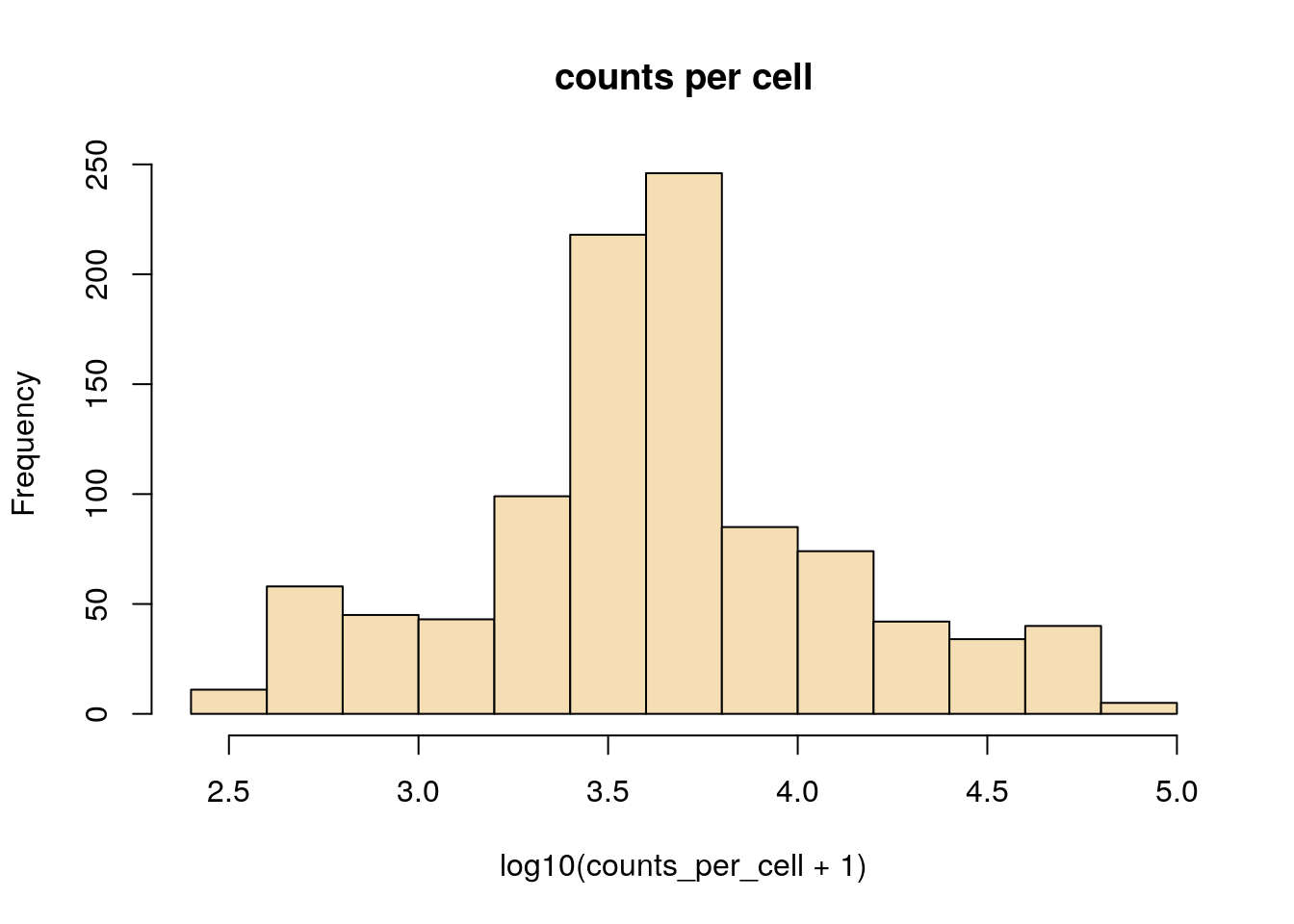
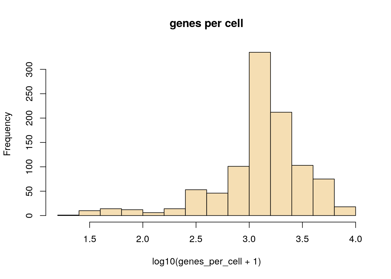
Here we see examples of plotting a new plot, the histogram. R makes this really easy with the hist function. We are also transforming the values to log10 before plotting, this is done with the log10 method. When logging count data, the + 1 is used to avoid log10(0) which is not defined.
Can you a histogram of counts per gene in log10 scale?
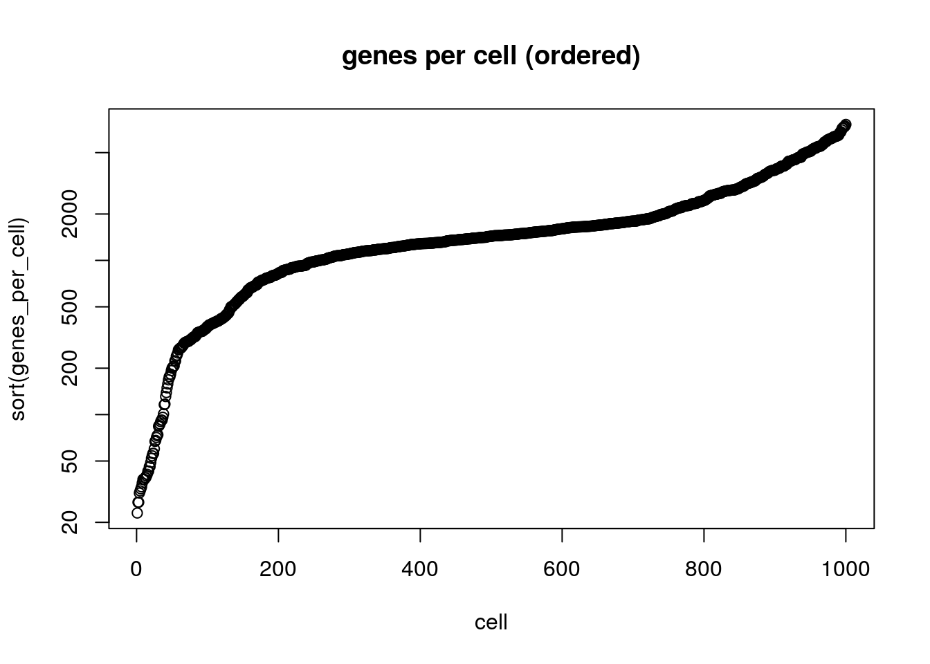
8.3.2 Plot cells ranked by their number of detected genes.
Here we rank each cell by its library complexity, ie the number of genes detected per cell. This is a very useful plot as it shows the distribution of library complexity in the sequencing run. One can use this plot to investigate observations (potential cells) that are actually failed libraries (lower end outliers) or observations that are cell doublets (higher end outliers).
8.4 Beginning with Seurat: http://satijalab.org/seurat/
8.4.1 Creating a seurat object
To analyze our single cell data we will use a seurat object. Can you create an Seurat object with the 10x data and save it in an object called ‘seurat’? hint: CreateSeuratObject(). Can you include only genes that are are expressed in 3 or more cells and cells with complexity of 350 genes or more? How many genes are you left with? How many cells?
## Warning: Feature names cannot have underscores ('_'), replacing with dashes
## ('-')Almost all our analysis will be on the single object, of class Seurat. This object contains various “slots” (designated by seurat@slotname) that will store not only the raw count data, but also the results from various computations below. This has the advantage that we do not need to keep track of inidividual variables of interest - they can all be collapsed into a single object as long as these slots are pre-defined.
The Assay class stores single cell data. For typical scRNA-seq experiments, a Seurat object will have a single Assay (“RNA”). This assay will also store multiple ‘transformations’ of the data, including raw counts ((???) slot), normalized data ((???) slot), and scaled data for dimensional reduction ((???) slot).
seurat@assays$RNA is a slot that stores the original gene count matrix. We can view the first 10 rows (genes) and the first 10 columns (cells).
## 10 x 10 sparse Matrix of class "dgCMatrix"## [[ suppressing 10 column names 'AAACCTGAGCTAGTCT', 'AAACCTGAGGGCACTA', 'AAACCTGAGTACGTTC' ... ]]##
## FO538757.2 . . . . 1 2 . . . .
## RP4-669L17.10 . . . . . . . . . .
## RP11-206L10.9 . . . . . . . . . .
## LINC00115 . . . . . . . . . .
## NOC2L . . . . 2 4 . 1 . .
## KLHL17 . . . . . . . . . .
## PLEKHN1 . . . . . . . . . .
## HES4 . . . . . 9 . . . 1
## ISG15 . . . . 1 1 . . 1 .
## AGRN . . . . . . . . . .8.5 Preprocessing step 1 : Filter out low-quality cells
The Seurat object initialization step above only considered cells that expressed at least 350 genes. Additionally, we would like to exclude cells that are damaged. A common metric to judge this (although by no means the only one) is the relative expression of mitochondrially derived genes. When the cells apoptose due to stress, their mitochondria becomes leaky and there is widespread RNA degradation. Thus a relative enrichment of mitochondrially derived genes can be a tell-tale sign of cell stress. Here, we compute the proportion of transcripts that are of mitochondrial origin for every cell (percent.mito), and visualize its distribution as a violin plot. We also use the GenePlot function to observe how percent.mito correlates with other metrics.
# The number of genes and UMIs (nGene and nUMI) are automatically calculated
# for every object by Seurat. For non-UMI data, nUMI represents the sum of
# the non-normalized values within a cell We calculate the percentage of
# mitochondrial genes here and store it in percent.mito using AddMetaData.
# We use object@raw.data since this represents non-transformed and
# non-log-normalized counts The % of UMI mapping to MT-genes is a common
# scRNA-seq QC metric.
mito.genes <- grep(pattern = "^MT-", x = rownames(x = seurat@assays$RNA@data), value = TRUE)
percent.mito <- Matrix::colSums(seurat@assays$RNA@data[mito.genes, ])/Matrix::colSums(seurat@assays$RNA@data)
# AddMetaData adds columns to object@meta.data, and is a great place to stash QC stats.
# This also allows us to plot the metadata values using the Seurat's VlnPlot().
head(seurat@meta.data) # Before adding## orig.ident nCount_RNA nFeature_RNA
## AAACCTGAGCTAGTCT 10X_NSCLC 3605 1184
## AAACCTGAGGGCACTA 10X_NSCLC 3828 1387
## AAACCTGAGTACGTTC 10X_NSCLC 6452 1783
## AAACCTGAGTCCGGTC 10X_NSCLC 3071 1088
## AAACCTGCACCAGGTC 10X_NSCLC 9389 2616
## AAACCTGCACCTCGTT 10X_NSCLC 48827 5591Task: Can you add the percentage if mitochondrial genes to the seurat object meta data? If you dont remember the name of the parameter you can type ?AddMetaData in the console. An alternative way to add meta data is by using: seurat[[“percent.mito”]] <- PercentageFeatureSet(seurat, pattern = “^MT-”)
seurat <- AddMetaData(object = seurat, ? = percent.mito, col.name = "percent.mito")
head(seurat@meta.data) # After adding
VlnPlot(object = seurat, features = c("nFeature_RNA", "nCount_RNA", "percent.mito"))Here we calculated the percent mitochondrial reads and added it to the Seurat object in the slot named meta.data. This allowed us to plot using the violin plot function provided by Seurat.
A third metric we use is the number of house keeping genes expressed in a cell. These genes reflect commomn processes active in a cell and hence are a good global quality measure. They are also abundant and are usually steadliy expressed in cells, thus less sensitive to the high dropout.
# Load the the list of house keeping genes
hkgenes <- read.table("data/resources/tirosh_house_keeping.txt", skip = 2)
hkgenes <- as.vector(hkgenes$V1)
# remove hkgenes that were not found
hkgenes.found <- which(toupper(rownames(seurat@assays$RNA@data)) %in% hkgenes)Task: 1. Sum the number of detected house keeping genes for each cell 2. Add this information as meta data to seurat 3. plot all metrics: “nGene”, “nUMI”, “percent.mito”,“n.exp.hkgenes” using VlnPlot
n.expressed.hkgenes <- ?(seurat@assays$RNA@data[hkgenes.found, ] > 0)
seurat <- AddMetaData(object = ?, ? = ?, col.name = "n.exp.hkgenes")
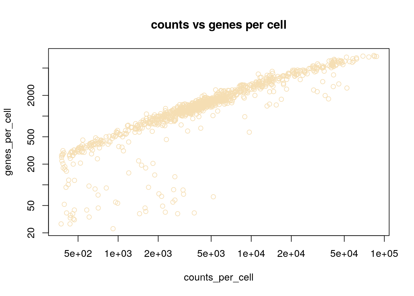
VlnPlot(object = seurat, features = c("nFeature_RNA", "nCount_RNA", "percent.mito","n.exp.hkgenes"), ncol = 4)Is there a correlation between the measurements? For example, number of UMIs with number of genes? Can you plot the nGene vs nUMI? What is the correlation? Do you see a strange subpopulation? What do you think happened with these cells?
8.6 Examine contents of Seurat object
These are the slots in the Seurat object. Some of the slots are automatically updated by Seurat as you move through analysis. Take a moment to look through the information, knowing the slots allow you to leverage work Seurat has already done for you.
Here we plot the number of genes per cell by what Seurat calls orig.ident. Identity is a concept that is used in the Seurat object to refer to the cell identity. In this case, the cell identity is 10X_NSCLC, but after we cluster the cells, the cell identity will be whatever cluster the cell belongs to. We will see how identity updates as we go throught the analysis.
Next, let’s filter the cells based on the quality control metrics. Filter based on: 1. nFeature_RNA 2. percent.mito 3. n.exp.hkgenes Task: Change the thresholds to what you think they should be according to the violin plots
## Warning in FetchData(object = object, vars = features, slot = slot): The
## following requested variables were not found: percent.mito, n.exp.hkgenes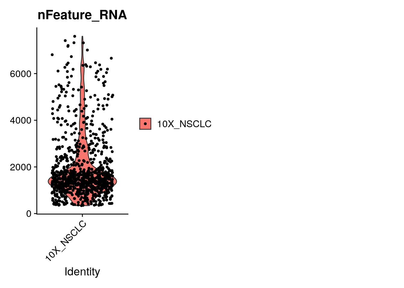
How many cells are you left with?
## An object of class Seurat
## 16145 features across 907 samples within 1 assay
## Active assay: RNA (16145 features)8.6.1 Preprocessing step 2 : Expression normalization
After removing unwanted genes cells from the dataset, the next step is to normalize the data. By default, we employ a global-scaling normalization method “LogNormalize” that normalizes the gene expression measurements for each cell by the total expression, multiplies this by a scale factor (10,000 by default), and log-transforms the result. There have been many methods to normalize the data, but this is the simplest and the most intuitive. The division by total expression is done to change all expression counts to a relative measure, since experience has suggested that technical factors (e.g. capture rate, efficiency of reverse transcription) are largely responsible for the variation in the number of molecules per cell, although genuine biological factors (e.g. cell cycle stage, cell size) also play a smaller, but non-negligible role. The log-transformation is a commonly used transformation that has many desirable properties, such as variance stabilization (can you think of others?).
Well there you have it! A filtered and normalized gene-expression data set. A great accomplishment for your first dive into scRNA-Seq analysis. Well done!
8.7 Detection of variable genes across the single cells
Seurat calculates highly variable genes and focuses on these for downstream analysis. FindVariableFeatures calculates the average expression and dispersion for each gene, places these genes into bins, and then calculates a z-score for dispersion within each bin. This helps control for the relationship between variability and average expression.
seurat <- FindVariableFeatures(seurat, selection.method = "vst", nfeatures = 2000)
# Identify the 10 most highly variable genes
top10 <- head(VariableFeatures(seurat), 10)
# plot variable features with and without labels
plot1 <- VariableFeaturePlot(seurat)
plot2 <- LabelPoints(plot = plot1, points = top10, repel = TRUE, xnudge = 0, ynudge = 0)## Warning: Using `as.character()` on a quosure is deprecated as of rlang 0.3.0.
## Please use `as_label()` or `as_name()` instead.
## This warning is displayed once per session.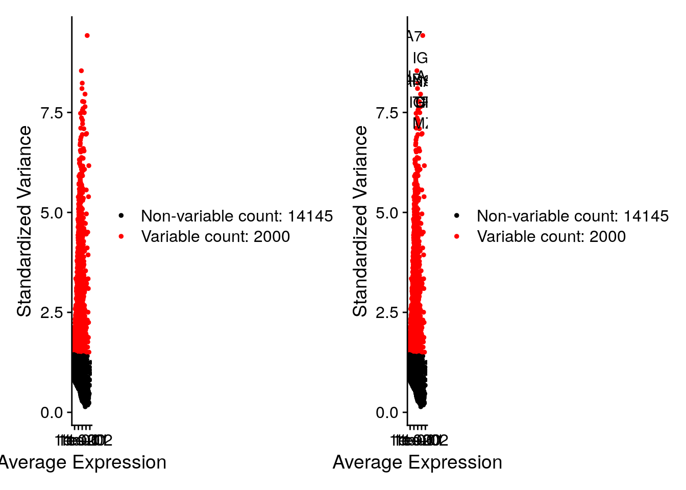
8.8 Gene set expression across cells
Sometimes we want to ask what is the expression of a set of a genes across cells. This set of genes may make up a gene expression program we are interested in. Another benefit at looking at gene sets is it reduces the effects of drop outs.
Below, we look at genes involved in: T cells, the cell cycle and the stress signature upon cell dissociation. We calculate these genes average expression levels on the single cell level, while controlling for technical effects.
# Read in a list of cell cycle markers, from Tirosh et al, 2015.
# We can segregate this list into markers of G2/M phase and markers of S phase.
cc.genes <- readLines("data/resources/regev_lab_cell_cycle_genes.txt")
s.genes <- cc.genes[1:43]
g2m.genes <- cc.genes[44:97]
seurat <- CellCycleScoring(seurat, s.features = s.genes, g2m.features = g2m.genes, set.ident = TRUE)## Warning: The following features are not present in the object: MLF1IP, not
## searching for symbol synonymsTask: Use markers for dissociation to calculate dissociation score
# Genes upregulated during dissociation of tissue into single cells.
genes.dissoc <- c("ATF3", "BTG2", "CEBPB", "CEBPD", "CXCL3", "CXCL2", "CXCL1", "DNAJA1", "DNAJB1", "DUSP1", "EGR1", "FOS", "FOSB", "HSP90AA1", "HSP90AB1", "HSPA1A", "HSPA1B", "HSPA1A", "HSPA1B", "HSPA8", "HSPB1", "HSPE1", "HSPH1", "ID3", "IER2", "JUN", "JUNB", "JUND", "MT1X", "NFKBIA", "NR4A1", "PPP1R15A", "SOCS3", "ZFP36")
#### seurat <- AddModuleScore(?, genes.list = list(?), ctrl.size = 20, enrich.name = "genes_dissoc")
seurat <- AddModuleScore(seurat, features = list(genes.dissoc), ctrl.size = 20, enrich.name = "genes_dissoc")Task: Plot the correlation between number of genes and S score. How do we know the name of these scores in the seurat meta data?
Congratulations! You can identify and visualize cell subsets and the marker genes that describe these cell subsets. This is a very powerful analysis pattern often seen in publications. Well done!
library(Seurat)
library(dplyr)
library(Matrix)
library(gdata)
# read data
dirname <- "/home/rstudio/data/"
counts_matrix_filename = paste0(dirname,"/filtered_gene_bc_matrices/GRCh38/")
counts <- Read10X(data.dir = counts_matrix_filename) # Seurat function to read in 10x count data
# To minimize memory use on the docker - choose only the first 1000 cells
counts <- counts[,1:1000]
# Let's examine the sparse counts matrix
counts[1:10, 1:3]
# How big is the matrix?
dim(counts) # report number of genes (rows) and number of cells (columns)
# How much memory does a sparse matrix take up relative to a dense matrix?
object.size(counts) # size in bytes
object.size(as.matrix(counts)) # size in bytes
# Look at the summary counts for genes and cells
counts_per_cell <- Matrix::colSums(counts)
counts_per_gene <- Matrix::rowSums(counts)
genes_per_cell <- Matrix::colSums(counts>0) # count gene only if it has non-zero reads mapped.
cells_per_gene <- Matrix::rowSums(counts>0) # only count cells where the gene is expressed
# plot counts and genes
hist(log10(counts_per_cell+1),main='counts per cell',col='wheat')
hist(log10(genes_per_cell+1), main='genes per cell', col='wheat')
plot(counts_per_cell, genes_per_cell, log='xy', col='wheat')
title('counts vs genes per cell')
# plot a histogram of counts per gene in log10 scale
hist(log10(counts_per_gene+1), main='counts per gene', col='wheat')
# Plot cells ranked by their number of detected genes.
plot(sort(genes_per_cell), xlab='cell', log='y', main='genes per cell (ordered)')
## Beginning with Seurat: http://satijalab.org/seurat/
# create object
seurat<-CreateSeuratObject(counts = counts, min.cells = 3, min.features = 350, project = "10X_NSCLC")
# vcalculate percent pf mitochondria genes
mito.genes <- grep(pattern = "^MT-", x = rownames(x = seurat@assays$RNA@data), value = TRUE)
percent.mito <- Matrix::colSums(seurat@assays$RNA@data[mito.genes, ])/Matrix::colSums(seurat@assays$RNA@data)
#### seurat <- AddMetaData(object = seurat, ? = percent.mito, col.name = "percent.mito")
seurat <- AddMetaData(object = seurat, metadata = percent.mito, col.name = "percent.mito")
head(seurat@meta.data) # After adding
VlnPlot(object = seurat, features = c("nFeature_RNA", "nCount_RNA", "percent.mito"))
# Load the the list of house keeping genes
hkgenes <- read.table("/home/rstudio/data/resources/tirosh_house_keeping.txt", skip = 2)
hkgenes <- as.vector(hkgenes$V1)
# remove hkgenes that were not found
hkgenes.found <- which(toupper(rownames(seurat@assays$RNA@data)) %in% hkgenes)
# Add_number_of_house_keeping_genes
n.expressed.hkgenes <- Matrix::colSums(seurat@assays$RNA@data[hkgenes.found, ] > 0)
seurat <- AddMetaData(object = seurat, metadata = n.expressed.hkgenes, col.name = "n.exp.hkgenes")
VlnPlot(object = seurat, features = c("nFeature_RNA", "nCount_RNA", "percent.mito","n.exp.hkgenes"), ncol = 4)
FeatureScatter(object = seurat, feature1 = "nFeature_RNA", feature2 = "nCount_RNA")
# plot seurat meta data
VlnPlot(object = seurat, features = c("nFeature_RNA"), group.by = c('orig.ident'))
VlnPlot(object = seurat, features = c("nFeature_RNA","percent.mito","n.exp.hkgenes"), ncol = 3)
# filter data
seurat <- subset(seurat, subset = nFeature_RNA > 350 & nFeature_RNA < 4000 & percent.mito < 0.15 & n.exp.hkgenes > 55)
#normalize
seurat <- NormalizeData(object = seurat, normalization.method = "LogNormalize", scale.factor = 1e4)
#find_var_genes
seurat <- FindVariableFeatures(seurat, selection.method = "vst", nfeatures = 2000)

# Identify the 10 most highly variable genes
top10 <- head(VariableFeatures(seurat), 10)

# plot variable features with and without labels
plot1 <- VariableFeaturePlot(seurat)
plot2 <- LabelPoints(plot = plot1, points = top10, repel = TRUE, xnudge = 0, ynudge = 0)
plot1 + plot2
#cell_cycle_genes
# Read in a list of cell cycle markers, from Tirosh et al, 2015.
# We can segregate this list into markers of G2/M phase and markers of S phase.
cc.genes <- readLines("/home/rstudio/data/resources/regev_lab_cell_cycle_genes.txt")
s.genes <- cc.genes[1:43]
g2m.genes <- cc.genes[44:97]
seurat <- CellCycleScoring(seurat, s.features = s.genes, g2m.features = g2m.genes, set.ident = TRUE)
#dissociation_signature
# Genes upregulated during dissociation of tissue into single cells.
genes.dissoc <- c("ATF3", "BTG2", "CEBPB", "CEBPD", "CXCL3", "CXCL2", "CXCL1", "DNAJA1", "DNAJB1", "DUSP1", "EGR1", "FOS", "FOSB", "HSP90AA1", "HSP90AB1", "HSPA1A", "HSPA1B", "HSPA1A", "HSPA1B", "HSPA8", "HSPB1", "HSPE1", "HSPH1", "ID3", "IER2", "JUN", "JUNB", "JUND", "MT1X", "NFKBIA", "NR4A1", "PPP1R15A", "SOCS3", "ZFP36")
seurat <- AddModuleScore(seurat, features = list(genes.dissoc), ctrl.size = 20, enrich.name = "genes_dissoc")
# correlation: cell cycle scoores and number of genes, eval = FALSE}
FeatureScatter(seurat, feature1 = "S.Score", "nFeature_RNA")