Introduction
This tutorial provides a practical, hands-on introduction to inferring developmental trajectories with Waddington-OT.
Single cell RNA-sequencing allows us to profile the diversity of cells along a developmental time-course by recording static snapshots at different time points $t_1, t_2, \ldots, t_T$. However, we cannot directly observe the progression of any individual cell over time because the measurement process is destructive.
Waddington-OT is designed to infer the temporal couplings of a developmental stochastic process $\mathbb{P}_t$ from samples collected independently at various time points. We represent a developing population of cells with a time-varying distribution $\mathbb{P}_t$ on gene expression space. The temporal couplings describe the flow of mass as the population develops and grows. For a pair of time points $(t_i,t_j)$, the coupling $\gamma_{t_i,t_j}$ tells us: What descendants does cell $x$ from time $t_i$ give rise to at time $t_j$?
In this tutorial, we explore the Waddington-OT workflow, starting with inferring temporal couplings with optimal transport. We then go through numerous downstream analyses including visualizing cell fates, interpolating the distribution of cells at held-out time points, and inferring gene regulatory networks. This page guides the reader through the concepts, each of which is illustrated with an interactive Jupyter notebook using data from a time-course of iPS reprogramming (Schiebinger et al. 2019).
The reader can follow along by either
- Downloading the notebooks and running the notebooks locally.
- Running the notebooks interactively online with Terra.
The tutorial input data contains an expression matrix and a file indicating the time of collection for each cell. The zip folder also contains the output of most intermediate computations, so the reader is (mostly) free to skip ahead to later notebooks without running all earlier notebooks. For this reason we also provide precomputed transport matrices (in a separate zip folder to reduce file sizes). Note that the expression matrix has been proprocessed by log-normalizing the raw count data (i.e. the units are log-tpm).
The tutorial is organized as follows. We begin by visualizing and exploring the data in Notebook 1. We then compute transport maps and infer temporal couplings in Notebooks 2 and 3. The next section is on interpreting transport maps. In Notebooks 4, 5, and 6 we visualizing fates and trajectories of sets of cells. In Notebook 7 we interpolate the distribution of cells at held-out time points, and in Notebook 8 we compute gene regulatory networks.
In addition to these notebooks, we also provide a command-line interface.
Visualizing and Exploring the Data
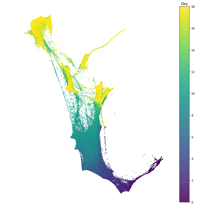
In this section we explore the time-series of reprogramming from Schiebinger et al. 2019. The dataset consists of 39 time points collected over 18 days of reprogramming. In the following notebook we visualize the dataset in two dimensions, and we examine patterns of gene expression programs.
Notebook 1: Visualizing and exploring the data
In this notebook we visualize the data with the force layout embedding. This is a graph visualization tool which we apply to layout a nearest neighbor graph constructed from our single cell gene expression data. There is a node for each cell, and each cell is connected to its $k$ nearest neighbors. Then the cells are arranged in 2D so that cells connected by an edge attract, and cells not connected by an edge repel each other. This visualization is used many times throughout the tutorial.
To get a basic idea of the lay of the land, we examine patterns of gene expression programs. To do this, we score each cell according to expression of a dictionary of gene signatures; in other words we test whether the set of genes in a signature is significantly expressed in each cell. Based on these gene signatures, we define sets of cells. In the following notebooks, we will use optimal transport to examine the developmental trajectories leading to these cell sets.
It's also possible to use the command-line interface to compute a FLE visualization of the data and to compute gene signature scores.
Inferring temporal couplings with optimal transport
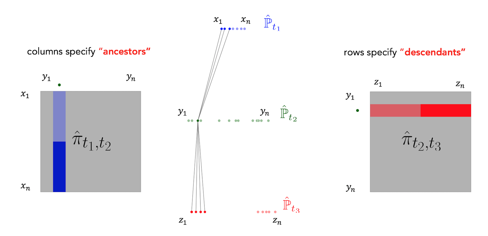
Waddington-OT infers temporal couplings by leveraging a classical mathematical tool called optimal transport. For each pair of adjacent time points $(t_k,t_{k+1})$, we compute a transport matrix $\pi_{t_i,t_{i+1}}$ connecting cells $x_1,\ldots,x_n$ at time $t_k$ to cells $y_1,\ldots, y_m$ at time $t_{k+1}$. To compute $\pi_{t_i,t_{i+1}}$, each cell $x_i$ at time $t_1$ is allocated a budget of descendant mass, and we seek to redistribute these descendants to the target cells $y_1, \ldots, y_m$ (which absorb mass $\frac 1 m$) in a way that minimizes the total transport cost (usually measured by mass $\times$ squared distance traveled). We then use the transport matrix $\pi_{t_k,t_{k+1}}$ as an estimate of the true temporal coupling $\gamma_{t_k,t_{k+1}}$: $$\pi_{t_k,t_{k+1}} \approx \gamma_{t_k,t_{k+1}}.$$ The transport matrix (a.k.a. 'transport map') tells us how many and what kind of descendants each cell from time $t_1$ would have at time $t_2$, if the measurement process hadn't killed the cell. Specifically, there is a row for each cell from time $t_1$ and a column for each cell from time $t_2$. Each row gives the descendant distribution of some cell $x_i$. The units of the transport map are 'descendant mass'. For example a value of $0.1$ in the $(x_i, y_j)$ entry means that cell $x_i$ will have on average $0.1$ descendants of type $y_j$ at time $t_2$.
Notebook 2: Computing transport matrices
In this notebook we compute transport matrices connecting each pair of time points, and we examine the effect of each parameter on the solution.
To compute the transport matrix $\pi_{t_1,t_2}$ connecting cells $x_1, \ldots, x_n$ at time $t_1$ to cells $y_1, \ldots, y_m$ at time $t_2$, we solve an optimization problem over all matrices $\pi$ that obey certain row-sum and column-sum constraints. These constraints ensure that the total amount of mass flowing out of each cell $x_i$ and into each cell $y_j$ adds up the correct amount. We select the transport matrix with the lowest possible transport cost, subject to these constraints.
We solve the following unbalanced transport optimization problem introduced in Chizat et al 2018, where we only enforce the row-sum constraints approximately and we add entropy to the transport matrix:
$$ \begin{aligned} \underset{\pi}{\text{minimize}} & \qquad \iint c(x,y) \pi(x,y) dx dy - \epsilon \int \pi(x,y) \log \pi(x,y) dx dy \\ &\qquad + \lambda_2 {\text{KL}} \left ( \int \pi(x,y) dx \Big \vert d \hat {\mathbb{P}}_{t_2} (y) \int g(x)^{t_2 - t_1} d \hat {\mathbb{P}}_{t_1}(x) \right ) \\ & \qquad + \lambda_1 {\text{KL}} \left ( \int \pi(x,y) dy \Big \vert d \hat {\mathbb{P}}_{t_1} (x) g(x)^{t_2 - t_1} \right). \end{aligned} $$
Here we use the notation $$\hat {\mathbb{P}}_{t_k} = \frac 1 n \sum_{i=1}^n \delta_{x_i}$$ for the empirical distribution of samples $x_1,\ldots,x_n$ at time $t_k$, and $\text{KL}(P \vert Q)$ denotes the KL-divergence between distributions $P$ and $Q$. The function $c(x,y)$ encodes the cost of transporting a unit mass from $x$ to $y$. We define $c(x,y)$ to be the squared euclidean distance between cells in local PCA space. This PCA space is computed separately for each pair of time points. Finally, the function $g(x)$ encodes the growth rate of cell $x$, and is used to specify the budget of descendant mass for each cell $x_i$ at time $t_1$.
The optimization problem has three regularization parameters:
- $\epsilon$ controls the degree of entropy in the transport map. A larger value gives more entropic descendant distributions, where cells are able to obtain more fates.
- $\lambda_1$ controls the constraint on the row sums of $\pi_{t_1,t_2}$, which depend on the growth rate function $g(x)$ A smaller value of $\lambda_1$ enforces the constraints less strictly, which is useful when we do not have precise information about $g(x)$.
- $\lambda_2$ controls the constraint on the column sums of $\pi_{t_1,t_2}$.
To define the growth rate function $g(x)$, we first form an initial estimate of cellular growth rates based on gene signatures of proliferation and apoptosis. We then refine this estimate using unbalanced optimal transport as follows. Because the row-sum constraints are not enforced strictly, the actual row-sums of the optimal transport map $\pi$ can be different than the initial input growth rate function $g$. We interpret these new row-sums as a meaningful estimate of growth rates, and use this to form a new estimate of the growth function $g^{(1)}$ which we can plug back into the OT optimization problem to compute a new transport map $\pi^{(1)}$. We can therefore iterate back and forth between learning growth rates $g^{(i)}$ and learning transport maps $\pi^{(i)}$ until the procedure eventually converges. In practice, we find that just a few iterations are usually sufficient.
It's also possible to use the command-line interface to compute transport maps.
Notebook 3: Inferring long-range temporal couplings
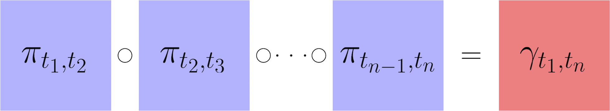
After having computed transport maps and used them to estimate the temporal couplings between adjacent time points, we next show how to infer transitions over a longer time interval $(t_i,t_j)$. To do this, we assume the developmental stochastic process is Markov. Therefore we can infer long-range transitions by composing transport maps as follows: $$\gamma_{t_i,t_j} = \gamma_{t_i,t_{i+1}} \circ \gamma_{t_{i+1},t_{i+2}} \circ \cdots \circ \gamma_{t_{j-1},t_{j}} \approx \pi_{t_i,t_{i+1}} \circ \pi_{t_{i+1},t_{i+2}} \circ \cdots \circ \pi_{t_{j-1},t_{j}}.$$ Here $\circ$ denotes matrix multiplication. The resulting temporal coupling $\gamma_{t_i,t_j}$ has a row for each cell at time $t_i$ and a column for each cell at time $t_j$. Just like for a short-range coupling, the units are 'transported mass'. So a value of $\gamma_{t_i,t_j}(x,y) = 1.2$ means that cell $x$ will have on average $1.2$ descendants with expression profile similar to $y$ at time $t_j$. The sum of the row shows the total number of descendants that a cell will have at time $t_j$.
Interpreting transport maps
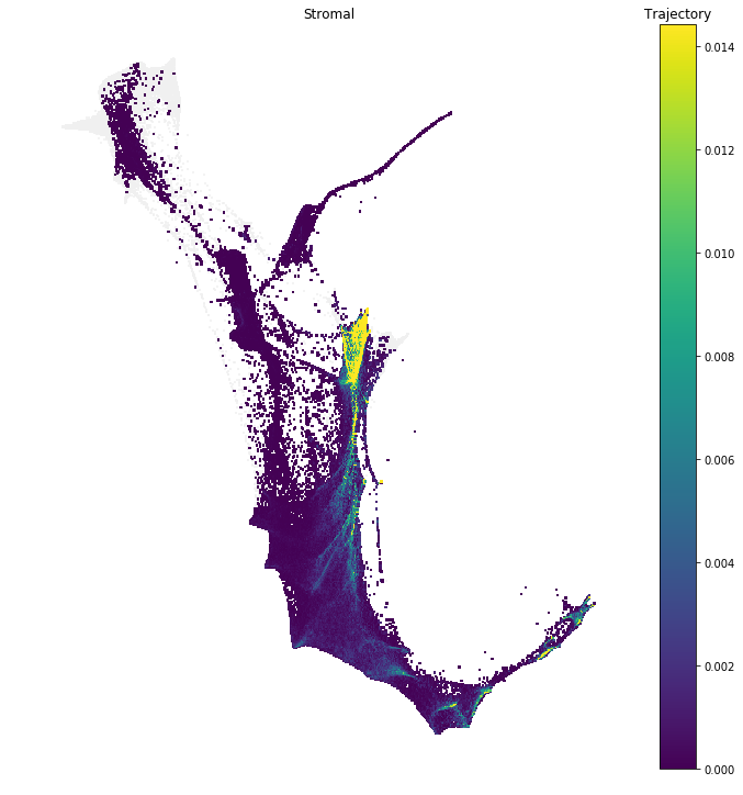
In this section we develop tools to interpret and visualize transport maps. Recall that in their raw form, the transport maps show the descendants and ancestors of each individual cell. Here we explore several different techniques to analyze the ancestors, descendants and trajectories of sets of cells.
Notebook 4: Ancestors descendants, and trajectories
We first describe how to compute the descendants of a set of cells.
Given a set $C$ of cells at time $t_j$, we can compute the descendant distribution at time $t_{j+1}$ by
pushing
the
cell set through the transport matrix.
This push forward operation is implemented in a matrix multiplication as follows. We first form the
probability
vector $p_{t_j}$ to represent the cell set $C$ as follows:
$$p_{t_j}(x) = \begin{cases} \frac 1 {|C|} & \quad x \in C \\ 0 & \quad \text{otherwise}\end{cases}.$$
Viewing this as a column vector, we push forward by multiplying by the transport map on the
right
$$p_{t_{j+1}}^T = p_{t_{j}}^T \pi_{t_j,t_{j+1}}.$$
We can then push $p_{t_{j+1}}$ forward again to compute the descendant distribution at the next time step.
Continuing in this way, we can compute the descendant distribution at any later time point $t_{\ell} > t_j$.
Note that this is equivalent to first forming the long-range coupling $\gamma_{t_j,t_\ell}$ and then pushing
$p_{t_j}$ forward according to this coupling:
$$p_{t_{\ell}}^T = p_{t_j}^T \gamma_{t_j,t_\ell}.$$
However, in practice it is faster to compute the descendant distribution with successive push-forward
operations,
each of which involves a matrix-vector multiplication. By contrast, forming the long-range coupling involves
matrix-matrix multiplies, which are significantly more expensive.
To compute the ancestors of $C$ at an earlier time point $t_i < t_j$, we pull the cell set
back
through the transport map.
This pull-back operation is also implemented as a matrix multiplication
$$p_{t_{j-1}} = \pi_{t_{j-1},t_j} p_{t_j}.$$
The trajectory of a cell set $C$ refers to the sequence of ancestor distributions at
earlier
time
points and descendant distributions at later time points.
In this notebook we explore tools to compute ancestor and descendant trajectories of cell sets, and also
several
tools to analyze these trajectories.
In particular, we show how to examine the shared ancestry between a pair of cell sets, to
study
when these two cell sets diverged from a common set of ancestors, and we show how to summarize an ancestor
trajectory in terms of an ancestor census. This census computes the amount of ancestor mass
contained in each of a number of descriptive cell sets.
It's also possible to use the command-line interface to compute trajectories, trajectory divergences, and expression trends.
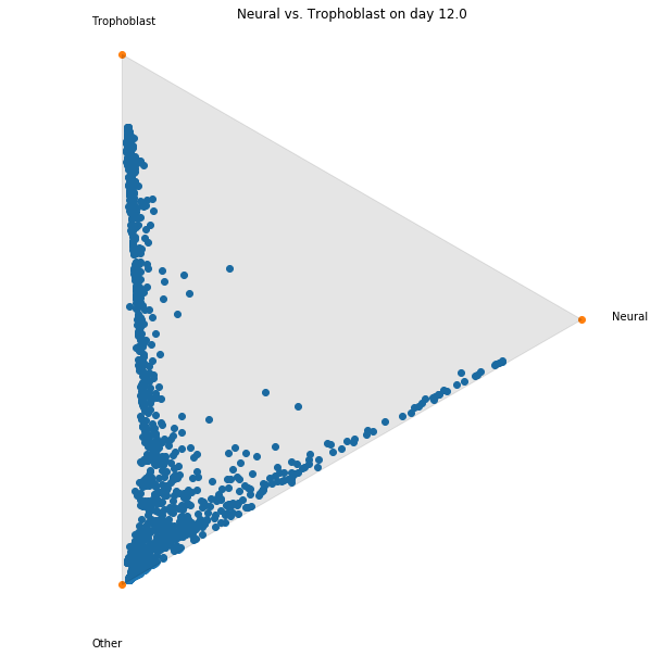
Notebook 5: Fate Matrices
In this notebook we show how to compute and visualize cell 'fates'.
Consider a pair of time points $t_i < t_j$ and a collection of cell sets $C_1,\ldots,C_k$ spanning all cells
at the later time point, $t_j$. (That is, each cell $y$ from time $t_j$ is in some $C_\ell$).
We show how to compute the probability that a cell $x$ from time $t_i$ will transition to a cell set
$C_\ell$ at
time $t_j$.
We call these the fate probabilities for cell $x$. The fate matrix $F_{t_i,t_j}$ is a
matrix
with a
row containing the fate probabilities for each cell $x$ from time $t_i$.
To compute the $F_{t_i,t_j}$, we take the long-range coupling $\gamma_{t_i,t_j}$ and first aggregate the
columns
according to the cell sets $C_1,\ldots, C_k$.
This yields an un-normalized fate matrix $\tilde F_{t_i,t_j}$:
$$\tilde F_{t_i,t_j}(x,\ell) = \sum_{y \in C_\ell} \gamma_{t_i,t_j}(x,y).$$
We then normalize each row to sum to $1$:
$$F_{t_i,t_j}(x,\ell) = \frac{\tilde F_{t_i,t_j}(x,\ell)}{\sum_{\ell = 1}^k \tilde F_{t_i,t_j}(x,\ell)}.$$
It's also possible to use the command-line interface to compute fate matrices.
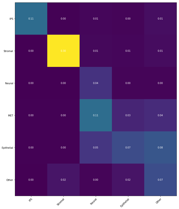
Notebook 6: Transition tables
Finally, if we have cell sets at both the beginning and ending time points, we can summarize the temporal
coupling
$\gamma_{t_i,t_j}$ in a 'transition table',
where we aggregate the transitions to show the transported mass between sets of cells.
This is very simple to compute! Suppose we have cell sets $A_1,A_2,A_3$ at time $t_1$ and cell sets
$B_1,B_2,B_3$ at
time $t_5$.
We can then compute a $3\times 3$ transition table to show the amount of mass transported from $A_i$ to
$B_j$
from
time $t_1$ to $t_5$ as follows:
$$ \text{mass transported from $A_i$ to $B_j$} \quad = \sum_{x \in A_i} \sum_{y \in B_j} \gamma_{t_1,t_5}
(x,y).$$
It's also possible to use the command-line interface to compute transition tables.
Validation and Experimental Design
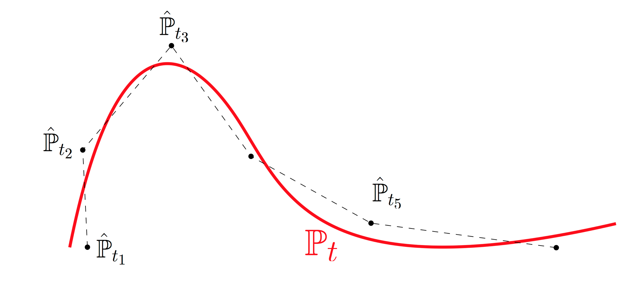
In this section we explain how to test whether temporal resolution is fine enough. This provides a rigorous basis for iterative experimental design: one can identify epochs without sufficient temporal resolution and collect additional samples in those intervals. Intuitively, the developmental process $\mathbb{P}_t$ traces out a curve in the space of distributions. We sample cells at various time points and obtain noisy samples along this curve. The empirical distributions $\hat{\mathbb{P}}_{t_i}$ don't lie precisely on the curve because we only have finitely many samples, and there are potential batch effects. Optimal transport allows us to connect these noisy samples with straight lines (aka geodesics or shortest paths) in the space of distributions. With fine enough time resolution, this piecewise-linear approximation provides a good fit. We can test the quality of fit by holding out time points and comparing our interpolation estimate to the real held-out data. The fit will be better when the time-resolution is shorter, but it won't ever be perfect because the measurements are inherently noisy. To quantify the baseline noise level, we compute the distance between two independent replicates at the same time point. When this noise level is comparable to our quality of interpolation, we have some reassurance that OT is working well.
Notebook 7: Validation by Geodesic Interpolation
In this notebook we apply the Waddington-OT Validation script to the reprogramming dataset. This script checks the quality of interpolation at each triplet of consecutive time points $(t_i,t_{i+1},t_{i+2})$:
- We hold out the data from time $t_{i+1}$,
- estimate the coupling $\gamma_{t_i,t_{i+2}}$ connecting time $t_{i}$ to $t_{i+2}$,
- compute an interpolating distribution at time $t_{i+1}$,
- and compare this to the held-out data $\hat{\mathbb{P}}_{t_{i+1}}$.
- If the held-out data consists of multiple batches (e.g. $\hat{\mathbb{P}}_{t_{i+1}}^{(1)}$ and $\hat{\mathbb{P}}_{t_{i+1}}^{(2)}$), then we compare those to eachother to estimate the baseline noise level.
It's also possible to use the command-line interface to run the validation script.
Inferring gene regulatory networks
In this section we show how to fit models of gene regulation to temporal couplings. Recall that the temporal coupling $\gamma_{t_1,t_2}$ defines a joint distribution between expression profiles at times $t_1$ and $t_2$. We can therefore sample pairs of points $(x_i,y_i)$ according to this joint distribution and use this as training data to fit a regulatory function $$y \approx f(x).$$ This idea can be implemented in different ways, depending on the class of functions we optimize over.
Notebook 8: Predictive TFs
One simple approach is to identify transcription factors that are predictive of subsequent fates. To do this, we construct the fate matrix and look for transcription factors that are enriched in cells most fated to transition to each particular fate.
It's also possible to use the command-line interface to identify differentially expressed transcription factors.