creating_merged

Last updated: 2019-12-17

Checks: 5 2

Knit directory: newlipids/

This reproducible R Markdown analysis was created with workflowr (version 1.4.0). The Checks tab describes the reproducibility checks that were applied when the results were created. The Past versions tab lists the development history.

R Markdown file: uncommitted changes

The R Markdown file has unstaged changes. To know which version of the R Markdown file created these results, you’ll want to first commit it to the Git repo. If you’re still working on the analysis, you can ignore this warning. When you’re finished, you can run wflow_publish to commit the R Markdown file and build the HTML.

Environment: empty

Great job! The global environment was empty. Objects defined in the global environment can affect the analysis in your R Markdown file in unknown ways. For reproduciblity it’s best to always run the code in an empty environment.

Seed: set.seed(20190925)

The command set.seed(20190925) was run prior to running the code in the R Markdown file. Setting a seed ensures that any results that rely on randomness, e.g. subsampling or permutations, are reproducible.

Session information: recorded

Great job! Recording the operating system, R version, and package versions is critical for reproducibility.

Cache: detected

The following chunks had caches available:

barplot
create table
mashblock
maxblock
posteriorblock
session-info-chunk-inserted-by-workflowr
unnamed-chunk-1
unnamed-chunk-2
unnamed-chunk-3
unnamed-chunk-4
unnamed-chunk-5
unnamed-chunk-6
unnamed-chunk-7
unnamed-chunk-8
zstuff

To ensure reproducibility of the results, delete the cache directory workingwithdata_cache and re-run the analysis. To have workflowr automatically delete the cache directory prior to building the file, set delete_cache = TRUE when running wflow_build() or wflow_publish().

File paths: relative

Great job! Using relative paths to the files within your workflowr project makes it easier to run your code on other machines.

Repository version: 392178a

Great! You are using Git for version control. Tracking code development and connecting the code version to the results is critical for reproducibility. The version displayed above was the version of the Git repository at the time these results were generated.

Note that you need to be careful to ensure that all relevant files for the analysis have been committed to Git prior to generating the results (you can use wflow_publish or wflow_git_commit). workflowr only checks the R Markdown file, but you know if there are other scripts or data files that it depends on. Below is the status of the Git repository when the results were generated:


Ignored files:
    Ignored:    .DS_Store
    Ignored:    analysis/.DS_Store
    Ignored:    analysis/.Rhistory
    Ignored:    analysis/looking_at_significance_cache/
    Ignored:    analysis/workingwithdata_cache/
    Ignored:    data/.DS_Store
    Ignored:    data/Archive.zip.gz
    Ignored:    data/Basic_mvp_sarah_HDL.tsv
    Ignored:    data/Basic_mvp_sarah_LDL.tsv
    Ignored:    data/Basic_mvp_sarah_LDL.tsv.zip
    Ignored:    data/Basic_mvp_sarah_TC.tsv
    Ignored:    data/Basic_mvp_sarah_TG.tsv
    Ignored:    data/EDcov.Rds
    Ignored:    data/EDcov_sim.Rds
    Ignored:    data/ash.rds
    Ignored:    data/ash_lf.txt
    Ignored:    data/ash_sim.rds
    Ignored:    data/gtexcolors.txt
    Ignored:    data/hdl_max.txt
    Ignored:    data/ldl_max.txt
    Ignored:    data/mashcomplete.rds
    Ignored:    data/mashcomplete.rds.zip
    Ignored:    data/mashresult_mvp.rds
    Ignored:    data/mashresult_sim.rds
    Ignored:    data/max_ld_block.txt
    Ignored:    data/merged_betas.txt
    Ignored:    data/merged_betas_mvp.txt
    Ignored:    data/merged_betas_mvp_simple.txt
    Ignored:    data/merged_p.txt
    Ignored:    data/merged_p_mvp_simple.txt
    Ignored:    data/merged_se.txt
    Ignored:    data/merged_se_mvp_simple.txt
    Ignored:    data/merged_z.txt
    Ignored:    data/merged_z_mvp.txt
    Ignored:    data/merged_z_mvp_withnames.txt
    Ignored:    data/tc_max.txt
    Ignored:    data/tg_max.txt
    Ignored:    data/znew.txt
    Ignored:    docs/.DS_Store
    Ignored:    docs/figure/.DS_Store

Unstaged changes:
    Modified:   analysis/simulations.Rmd
    Modified:   analysis/workingwithdata.Rmd

Note that any generated files, e.g. HTML, png, CSS, etc., are not included in this status report because it is ok for generated content to have uncommitted changes.

These are the previous versions of the R Markdown and HTML files. If you’ve configured a remote Git repository (see ?wflow_git_remote), click on the hyperlinks in the table below to view them.

File	Version	Author	Date	Message
Rmd	52c52c7	Sarah Urbut	2019-11-01	Update
Rmd	76cc40a	Sarah Urbut	2019-10-27	Update
html	76cc40a	Sarah Urbut	2019-10-27	Update
Rmd	3f85586	Sarah Urbut	2019-10-07	Update
html	3f85586	Sarah Urbut	2019-10-07	Update
Rmd	079589b	Sarah Urbut	2019-10-07	Update
html	079589b	Sarah Urbut	2019-10-07	Update
Rmd	7142cc6	Sarah Urbut	2019-10-04	Updated plots
html	7142cc6	Sarah Urbut	2019-10-04	Updated plots
Rmd	73da9ad	Sarah Urbut	2019-10-03	Update
html	73da9ad	Sarah Urbut	2019-10-03	Update
html	ca158bf	Sarah Urbut	2019-10-03	Update docs

R Markdown

Here we will try to merge based on common chr.position (per Hg18) names.

To run mashr, we need a matrix of maxes. The best way to do this is to choose the max effect across conditions per LD block, as described in Pickrell et al. Only then can we assume the maxes used to create covariance matrices are truly linearly independent. We will select SNPS falling within each of the 1700 LD blocks and choose SNP with maximum absolute effect acrtoss conditions.

ztab=read.table("~/lipids_mvp/data/merged_z_mvp_withnames.txt")
bed=read.table("~/Downloads/ld_chunk.bed")
head(bed)

    V1      V2      V3
1 chr1   10583 1892607
2 chr1 1892607 3582736
3 chr1 3582736 4380811
4 chr1 4380811 5913893
5 chr1 5913893 7247335
6 chr1 7247335 9365199

maxes=apply(ztab[,c("beta.x","beta.y","tgbeta","tcbeta")],1,function(x){max(abs(x))})
znew=cbind(ztab,maxes)
colnames(znew)[c(4:7)]=c("hdl","ldl","tg","tc")

max_block=data.frame(matrix(ncol = ncol(znew), nrow = nrow(bed)))
colnames(max_block)=colnames(znew)
for(i in 1:nrow(bed)){
  chr=bed[i,1]
  start=bed[i,2]
  stop=bed[i,3]
  in_chrom=znew[znew$hg19chrc==chr,]
  goodguys=in_chrom[in_chrom$bp>start&in_chrom$bp<stop,]
 if(nrow(goodguys)>0) {
    z.max=which.max(goodguys[,"maxes"])
    z_good=goodguys[z.max,]
    } else {
      z_good=rep(0,ncol(max_block))
    }
  z_good=data.table(z_good,stringsAsFactors = T)
  z_good$hg19chrc=as.character(z_good$hg19chrc)
  z_good$snpid.x=as.character(z_good$snpid.x)
  max_block[i,]=z_good
  print(i)
}

max_block=na.omit(max_block)
write.table(max_block,"~/lipids_mvp/data/max_ld_block.txt")

Now, we’re ready to mash!

ztab=read.table("~/lipids_mvp/data/merged_z_mvp_withnames.txt")
znew=read.table("~/lipids_mvp/data/merged_z_mvp.txt")
colnames(znew)=c("hdl","ldl","tg","tc")
library("mashr")
library("flashr")
max_block=read.table("~/lipids_mvp/data/max_ld_block.txt")
source('~/Dropbox/jointData/flashscript.R')
# identify a random subset of 20000 tests
random.subset = sample(1:nrow(znew),40000)
zmash=as.matrix(znew[,c("hdl","ldl","tg","tc")]);rownames(zmash)=ztab$snpid.x
data.temp = mash_set_data(zmash[random.subset,],alpha = 1)
Vhat = estimate_null_correlation_simple(data.temp)
saveRDS("~/lipids_mvp/data/MVPVhat.rds")
library("lattice")
clrs = colorRampPalette((c("#D73027","#FC8D59","#FEE090","#FFFFBF", "#E0F3F8","#91BFDB","#4575B4")))(64)

print(levelplot(Vhat,col.regions = clrs,xlab = "",ylab = "",colorkey = TRUE,main="VHAT"))

rm(data.temp)
data.random = mash_set_data(zmash[random.subset,],alpha = 1,V=Vhat)

zmax=apply(max_block[,c(4:7)],2,function(x){as.numeric(x)});rownames(zmax)=max_block$snpid.x
data.strong = mash_set_data(zmax,alpha = 1,V=Vhat)

U.pca = cov_pca(data.strong,3)

U.flash=cov_flash(data.strong, non_canonical = TRUE)
X.center = apply(data.strong$Bhat, 2, function(x) x - mean(x))
U.ed = cov_ed(data.strong, c(U.flash, U.pca, list("XX" = t(X.center) %*% X.center / nrow(X.center))))
saveRDS(U.ed,"~/lipids_mvp/data/EDcov.Rds")

U.ed=readRDS("~/lipids_mvp/data/EDcov.Rds")
U.c = cov_canonical(data.random)
m = mash(data.random, Ulist = c(U.ed,U.c),outputlevel = 1)
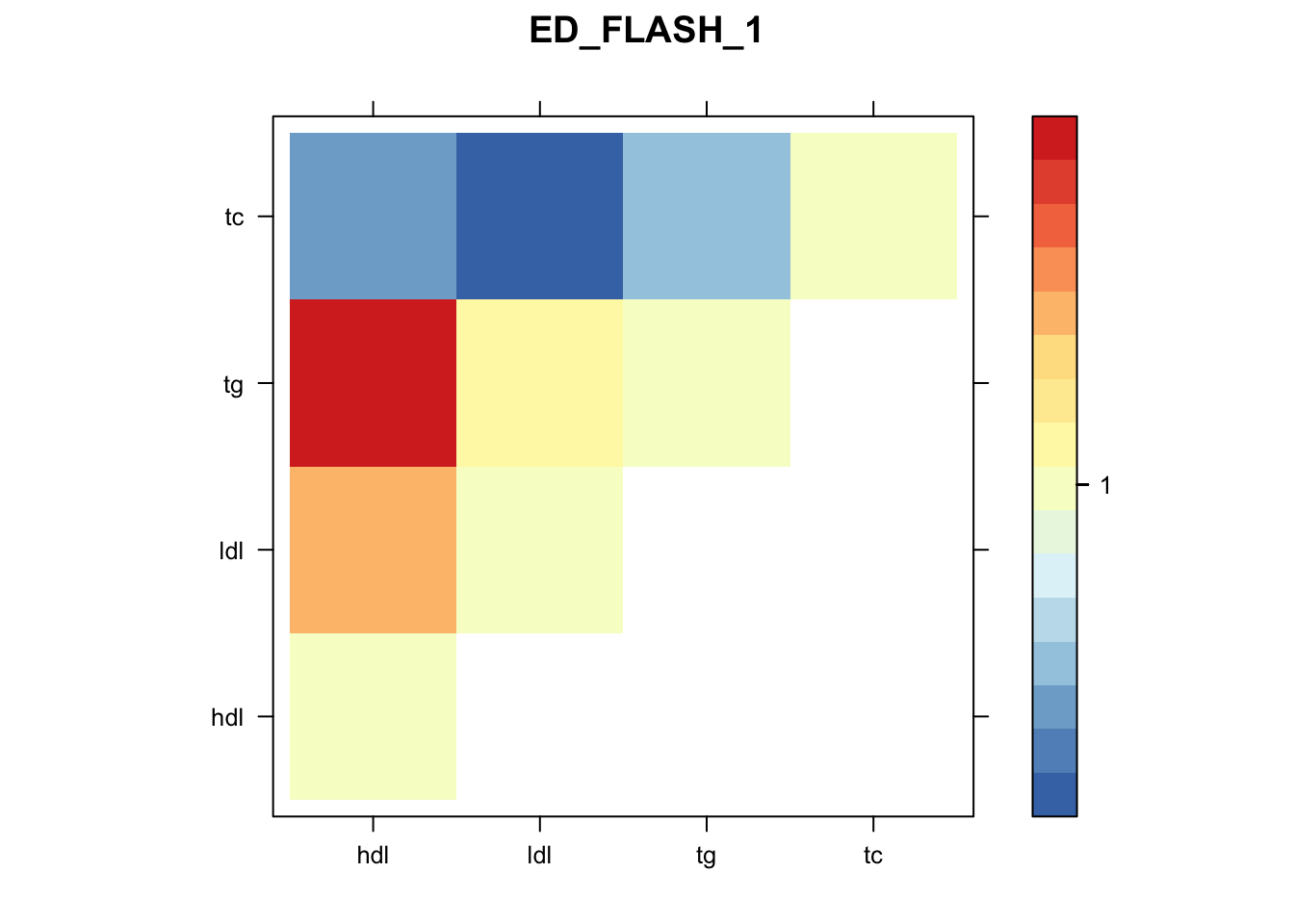
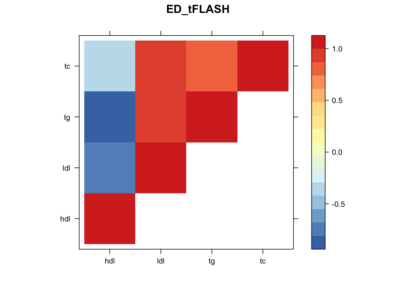
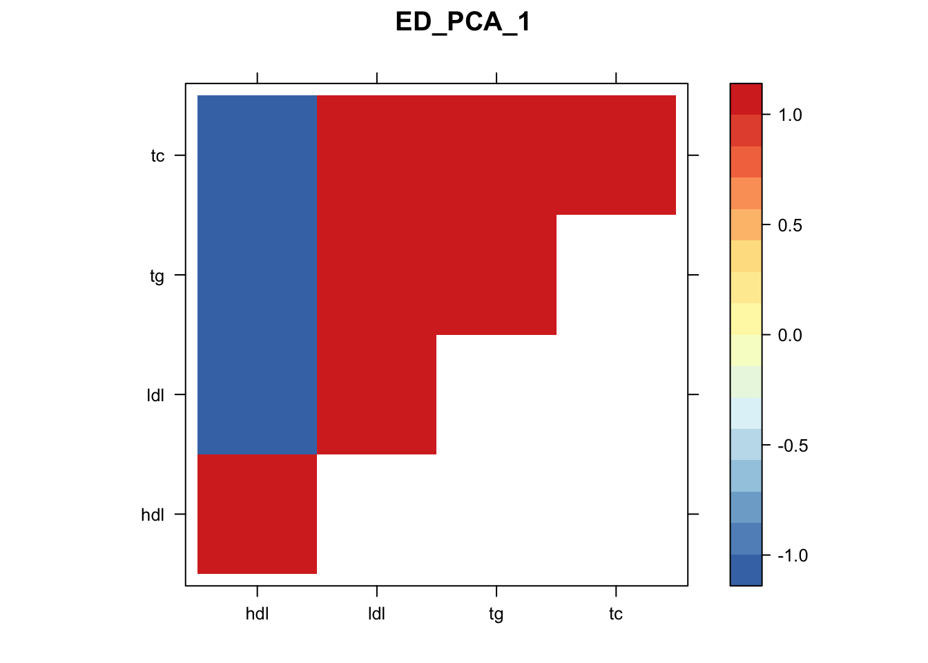
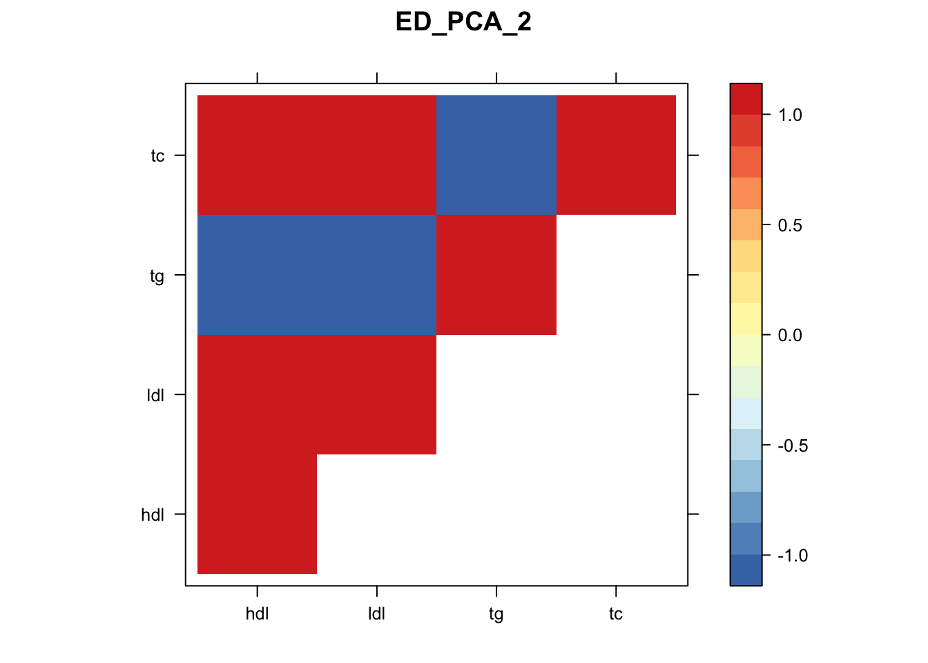
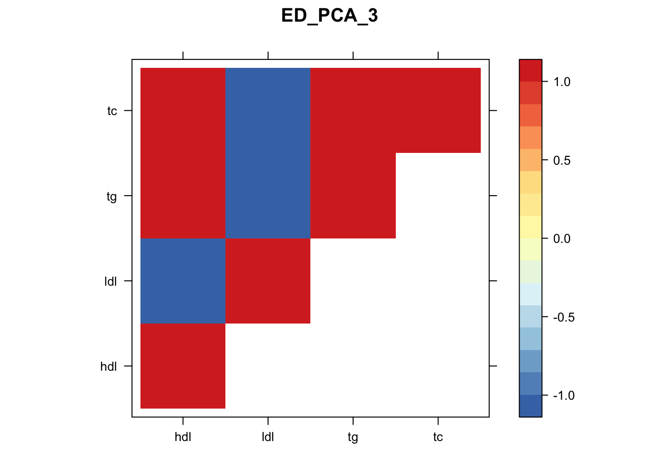
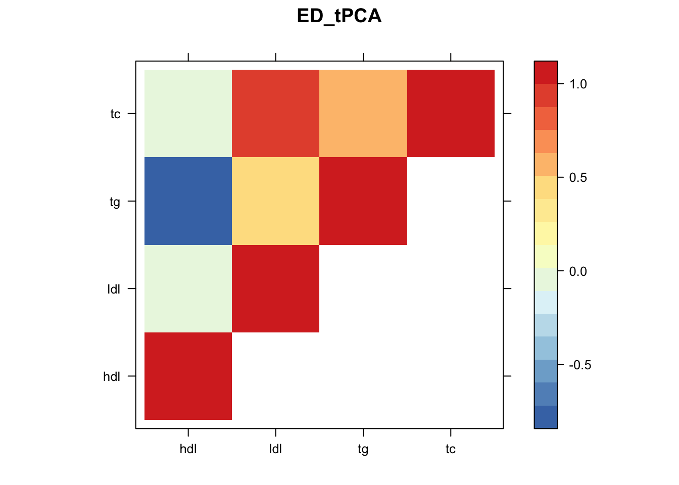
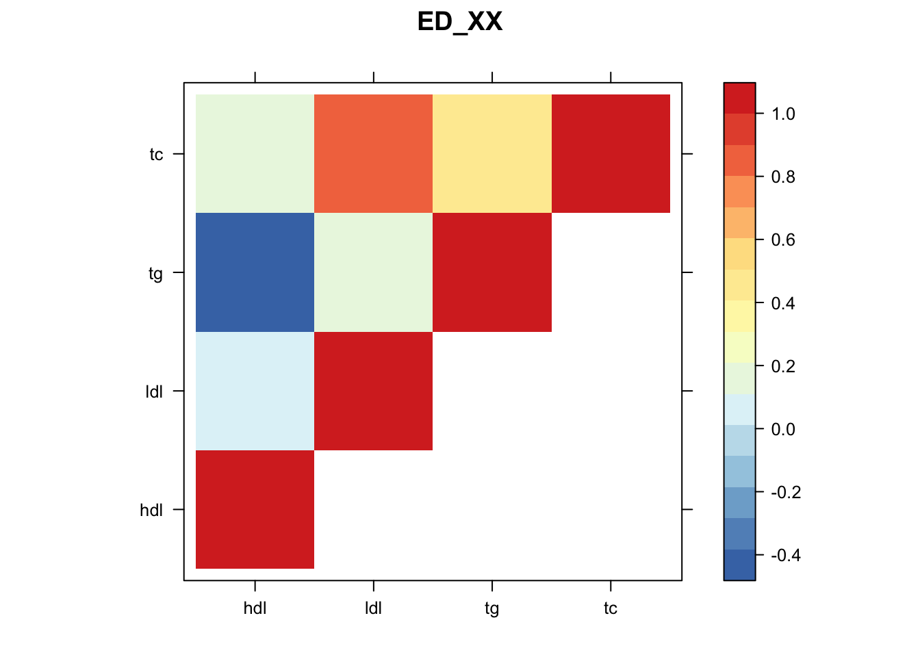
saveRDS(m,"~/lipids_mvp/data/mfitMVP.rds")

Now, let’s plot the patterns of sharing as the correlation matrix of the estimated covariance matrices..

zmash=read.table("~/lipids_mvp/data/merged_z_mvp.txt")
colnames(zmash)=c("hdl","ldl","tg","tc")

m=readRDS("~/lipids_mvp/data/mfitMVP.rds")

k=length(m$fitted_g$Ulist)
l=length(m$fitted_g$grid)
pimat=matrix(m$fitted_g$pi[-1],nrow=l,byrow=T)
colnames(pimat)=names(m$fitted_g$pi)[2:(k+1)]
barplot(colSums(pimat),las=2)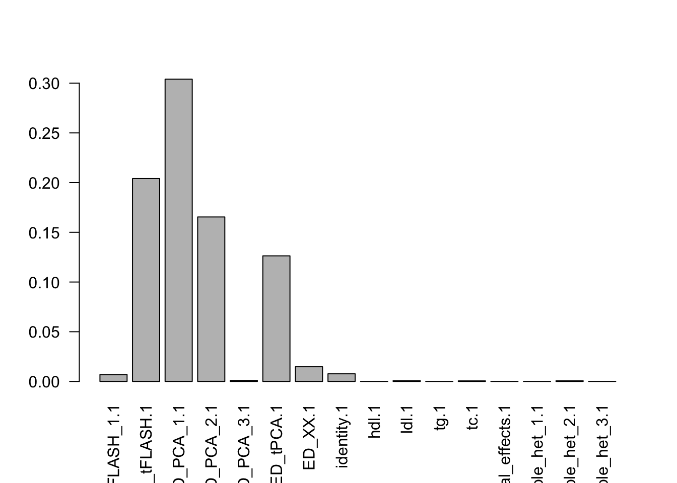

Version	Author	Date
76cc40a	Sarah Urbut	2019-10-27

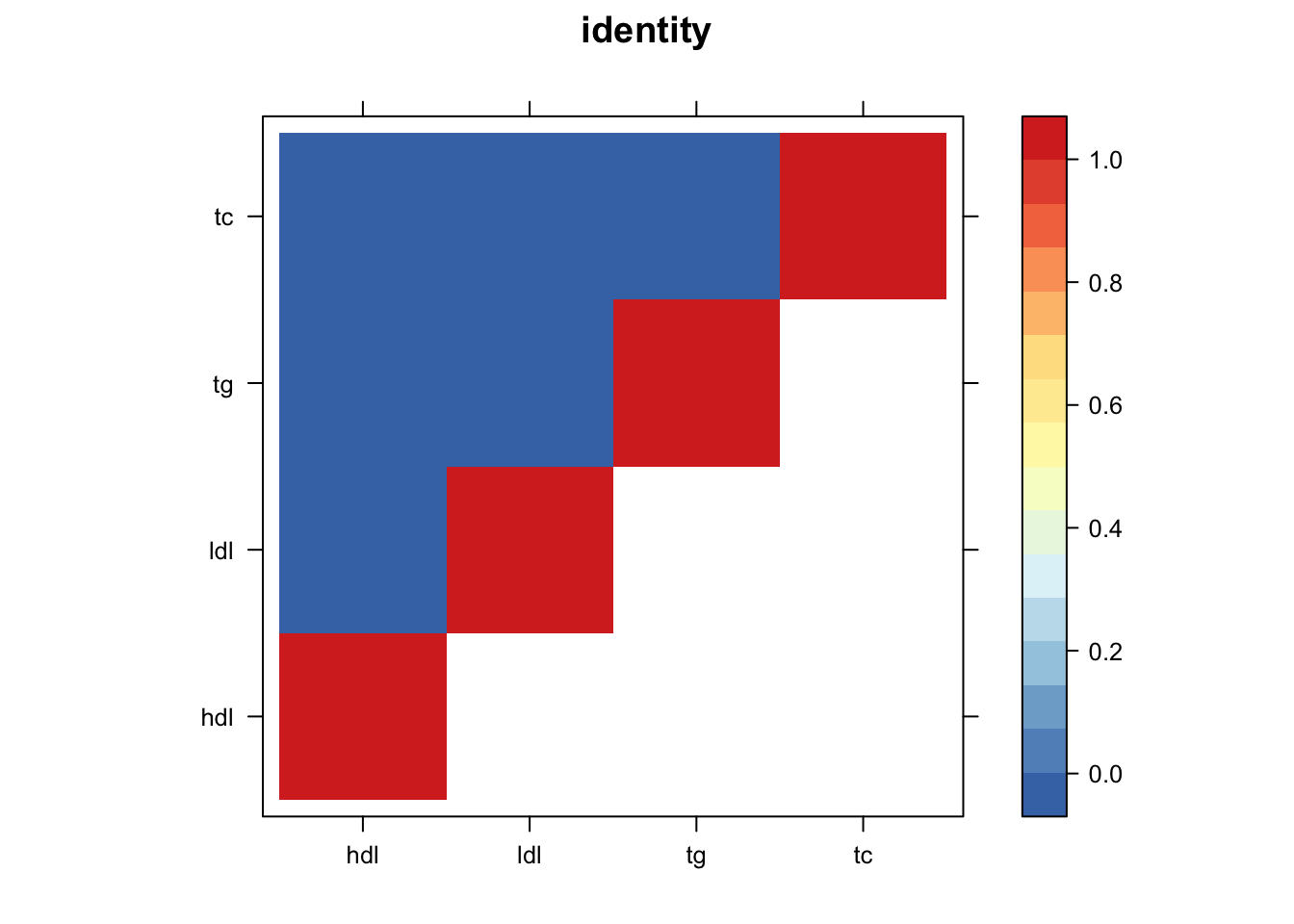
library("lattice")
for(i in 1:8){
  z.num=as.matrix(cov2cor(m$fitted_g$Ulist[[i]]))
  colnames(z.num)=row.names(z.num)=colnames(zmash)
clrs = colorRampPalette(rev(c("#D73027","#FC8D59","#FEE090","#FFFFBF", "#E0F3F8","#91BFDB","#4575B4")))(64)
z.num[lower.tri(z.num)] = NA
print(levelplot(z.num,col.regions = clrs,xlab = "",ylab = "",colorkey = TRUE,main=paste0(names(m$fitted_g$Ulist)[[i]])))
}

Version	Author	Date
76cc40a	Sarah Urbut	2019-10-27

Version	Author	Date
76cc40a	Sarah Urbut	2019-10-27

Version	Author	Date
76cc40a	Sarah Urbut	2019-10-27

Version	Author	Date
76cc40a	Sarah Urbut	2019-10-27

Version	Author	Date
76cc40a	Sarah Urbut	2019-10-27

Version	Author	Date
76cc40a	Sarah Urbut	2019-10-27

Version	Author	Date
76cc40a	Sarah Urbut	2019-10-27

Version	Author	Date
76cc40a	Sarah Urbut	2019-10-27

Now we can compute posteriors,

mash.data=mash_set_data(zmash,V = Vhat,alpha = 1)

m$result=mash_compute_posterior_matrices(m, mash.data, algorithm.version = "Rcpp")
saveRDS(m,"~/lipids_mvp/data/mashresult_mvp.rds")

Let’s take a look:

m=readRDS("~/lipids_mvp/data/mashresult_mvp.rds")
head(m$result$PosteriorMean)

                   hdl         ldl         tg          tc
rs6678176    1.0629093  0.07148775 -0.8411636  0.04103405
rs76909621   0.3901428 -0.18927773 -0.4152670 -0.21156310
rs78642210   0.1458664  0.07404952 -0.1182961  0.05731219
rs77140576   0.3656539 -0.18871989 -0.3827297 -0.20549333
rs113470118 -0.1377051 -0.07017948  0.1158224 -0.05287451
rs75635821   0.3603703 -0.18449444 -0.3773584 -0.20126912

head(m$result$lfsr)

                  hdl       ldl        tg        tc
rs6678176   0.1123920 0.4741408 0.1205983 0.5169807
rs76909621  0.2961115 0.4053798 0.3025860 0.4295731
rs78642210  0.4989478 0.5404176 0.4937694 0.5447642
rs77140576  0.3110436 0.4119177 0.3205846 0.4379812
rs113470118 0.5039852 0.5445682 0.4971376 0.5495551
rs75635821  0.3143522 0.4154700 0.3236874 0.4409992

lfsr=m$result$lfsr
s=rowSums(lfsr<=0.05)

hist(s[s>1],freq=FALSE,main="Number of Conditions")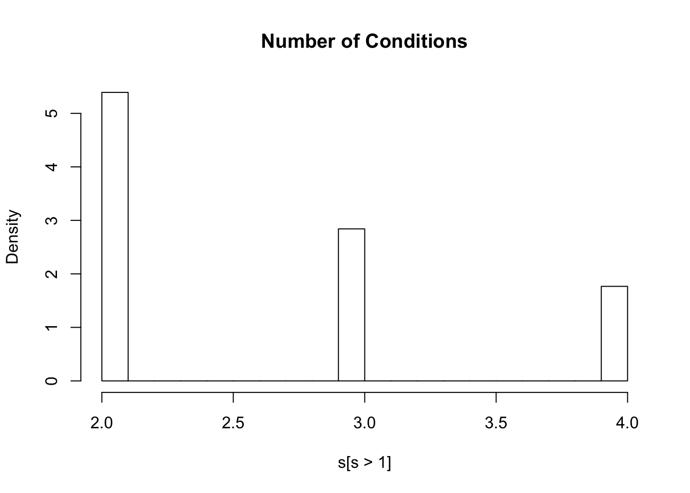

Version	Author	Date
76cc40a	Sarah Urbut	2019-10-27

#ash.z=apply(zmash,2,function(x){ashr::ash(x,sebetahat = rep(1,length(x)))})
# ash.pm=matrix(nrow=nrow(zmash),ncol=ncol(zmash))
# ash.lf=matrix(nrow=nrow(zmash),ncol=ncol(zmash))
# 
# for(i in 1:ncol(zmash))
#   
# {
#   x=zmash[,i]
#   a=ashr::ash(x,sebetahat = rep(1,length(x)))
#   ash.pm[,i]=a$result$PosteriorMean
#   ash.lf[,i]=a$result$lfsr
#   print(i)
# }
# 
# 
# colnames(ash.pm)=colnames(ash.lf)=colnames(zmash)
# rownames(ash.pm)=rownames(ash.lf)=rownames(zmash)
# 
# write.table(ash.pm,"~/lipids_mvp/data/ash_pm.txt")
# write.table(ash.lf,"~/lipids_mvp/data/ash_lf.txt")

ash.lf=read.table("~/lipids_mvp/data/ash_lf.txt")

ptab=apply(zmash,2,function(x){2*pnorm(-abs(x))})
#write.table(ptab,"~/lipids_mvp/data/merged_p.txt")
sum(ash.lf<0.05)

[1] 106052

sum(lfsr<0.05)

[1] 237730

Here 106052 SNPS x Conditions are less than 0.05 using a univariate appropach and 237730 are less than 0.05 with a joint approach, a roughly 250% increase. Furthermore, 102253 SNPS are significant in at least one condition wiht a juint approach, while 72875 with a univariate one.

p=read.table("~/lipids_mvp/data/merged_p.txt")
library(knitr)
library(kableExtra)
dt <- cbind(c(paste("Bonferroni=",sum(p<=5e-8)),paste("univariate_ash=",sum(ash.lf<0.05)),paste("mv_mash=",sum(lfsr<0.05))))

dt <- cbind(c(sum(p<=5e-8),sum(ash.lf<0.05),sum(lfsr<0.05)))
dt=cbind(dt,c(sum(rowSums(p<=5e-8)>0),sum(rowSums(ash.lf<0.05)>0),sum(rowSums(lfsr<0.05)>0)))
rownames(dt)=c("Bonferroni","UnivariateAsh","Mash")
colnames(dt)=c("Overall All Associations","Per Snp, in at least one")           
              
kable(dt)

	Overall All Associations	Per Snp, in at least one
Bonferroni	25260	16843
UnivariateAsh	106052	72875
Mash	237730	102253

dt %>%
  kable() %>%
  kable_styling()

	Overall All Associations	Per Snp, in at least one
Bonferroni	25260	16843
UnivariateAsh	106052	72875
Mash	237730	102253

sessionInfo()

R version 3.5.2 (2018-12-20)
Platform: x86_64-apple-darwin15.6.0 (64-bit)
Running under: macOS Mojave 10.14.6

Matrix products: default
BLAS: /Library/Frameworks/R.framework/Versions/3.5/Resources/lib/libRblas.0.dylib
LAPACK: /Library/Frameworks/R.framework/Versions/3.5/Resources/lib/libRlapack.dylib

locale:
[1] en_US.UTF-8/en_US.UTF-8/en_US.UTF-8/C/en_US.UTF-8/en_US.UTF-8

attached base packages:
[1] stats     graphics  grDevices utils     datasets  methods   base     

other attached packages:
[1] lattice_0.20-38   flashr_0.6-3      mashr_0.2.21.0631 ashr_2.2-37      
[5] reshape_0.8.8    

loaded via a namespace (and not attached):
 [1] Rcpp_1.0.1        pillar_1.4.2      compiler_3.5.2   
 [4] git2r_0.26.1      plyr_1.8.4        highr_0.8        
 [7] workflowr_1.4.0   iterators_1.0.10  tools_3.5.2      
[10] digest_0.6.20     tibble_2.1.3      gtable_0.3.0     
[13] evaluate_0.14     pkgconfig_2.0.2   rlang_0.4.0      
[16] Matrix_1.2-17     foreach_1.4.4     rstudioapi_0.10  
[19] yaml_2.2.0        parallel_3.5.2    mvtnorm_1.0-11   
[22] xfun_0.8          dplyr_0.8.3       stringr_1.4.0    
[25] knitr_1.23        fs_1.3.1          tidyselect_0.2.5 
[28] rprojroot_1.3-2   grid_3.5.2        glue_1.3.1       
[31] R6_2.4.0          rmarkdown_1.14    mixsqp_0.1-97    
[34] rmeta_3.0         reshape2_1.4.3    purrr_0.3.2      
[37] ggplot2_3.2.0     magrittr_1.5      scales_1.0.0     
[40] backports_1.1.4   codetools_0.2-16  htmltools_0.3.6  
[43] MASS_7.3-51.4     abind_1.4-5       assertthat_0.2.1 
[46] softImpute_1.4    colorspace_1.4-1  stringi_1.4.3    
[49] lazyeval_0.2.2    munsell_0.5.0     doParallel_1.0.14
[52] pscl_1.5.2        truncnorm_1.0-8   SQUAREM_2017.10-1
[55] crayon_1.3.4

creating_merged_lipids

R Markdown