TORUS
Last updated: 2021-12-16
Checks: 6 1
Knit directory: natarajanlab_wiki/
This reproducible R Markdown analysis was created with workflowr (version 1.6.2). The Checks tab describes the reproducibility checks that were applied when the results were created. The Past versions tab lists the development history.
The R Markdown file has unstaged changes. To know which version of the R Markdown file created these results, you’ll want to first commit it to the Git repo. If you’re still working on the analysis, you can ignore this warning. When you’re finished, you can run wflow_publish to commit the R Markdown file and build the HTML.
Great job! The global environment was empty. Objects defined in the global environment can affect the analysis in your R Markdown file in unknown ways. For reproduciblity it’s best to always run the code in an empty environment.
The command set.seed(20210512) was run prior to running the code in the R Markdown file. Setting a seed ensures that any results that rely on randomness, e.g. subsampling or permutations, are reproducible.
Great job! Recording the operating system, R version, and package versions is critical for reproducibility.
Nice! There were no cached chunks for this analysis, so you can be confident that you successfully produced the results during this run.
Great job! Using relative paths to the files within your workflowr project makes it easier to run your code on other machines.
Great! You are using Git for version control. Tracking code development and connecting the code version to the results is critical for reproducibility.
The results in this page were generated with repository version aca2bdc. See the Past versions tab to see a history of the changes made to the R Markdown and HTML files.
Note that you need to be careful to ensure that all relevant files for the analysis have been committed to Git prior to generating the results (you can use wflow_publish or wflow_git_commit). workflowr only checks the R Markdown file, but you know if there are other scripts or data files that it depends on. Below is the status of the Git repository when the results were generated:
Ignored files:
    Ignored:    .DS_Store
    Ignored:    .Rhistory
    Ignored:    analysis/.Rhistory
    Ignored:    analysis/lfsr vs logEFfect.png
    Ignored:    analysis/metaplot_strat_torus.nb.html
    Ignored:    analysis/monster_mash.nb.html
    Ignored:    analysis/prs_equivalency.nb.html
    Ignored:    analysis/testplot.nb.html

Untracked files:
    Untracked:  analysis/ash_mash_comp.Rmd
    Untracked:  analysis/metatrials_sim.Rmd
    Untracked:  analysis/prs_early_cad.Rmd
    Untracked:  analysis/testplot.Rmd
    Untracked:  analysis/torus.Rmd

Unstaged changes:
    Modified:   analysis/metaplot_strat_torus.Rmd
    Modified:   analysis/prs_equivalency.Rmd
    Modified:   analysis/venn_diagrams.Rmd
Note that any generated files, e.g. HTML, png, CSS, etc., are not included in this status report because it is ok for generated content to have uncommitted changes.
These are the previous versions of the repository in which changes were made to the R Markdown (analysis/metaplot_strat_torus.Rmd) and HTML (docs/metaplot_strat_torus.html) files. If you’ve configured a remote Git repository (see ?wflow_git_remote), click on the hyperlinks in the table below to view the files as they were in that past version.
| File | Version | Author | Date | Message |
|---|---|---|---|---|
| html | 8438818 | Your Name | 2021-09-04 | update metaplot |
| html | 2a8591f | Your Name | 2021-09-04 | removed |
| Rmd | b273764 | Your Name | 2021-09-04 | Update |
| html | a3d2e18 | Your Name | 2021-09-03 | update trous |
Introduction
We seek to quantify the enrichment of annotation parameters using multivariate or univariate input. To run the software TORUS we use a pipeline available using the workflow manager SOS and run the following two lines of code.
sos run fine-mapping/gwas_enrichment.ipynb range2var_annotation --cwd $work_dir --annotation_dir $anno_dir --z-score $z_file --single-annot $single
sos run fine-mapping/gwas_enrichment.ipynb enrichment --cwd $work_dir --annotation_dir $anno_dir --z-score $z_file --single-annot $single --blocks $blk --snps $snps
We place the results of the Torus pipeline in mvp_complete_torus where mash and original refer to the results using univariate and multivariate summary stats respectively.
Here, we plot the meta analysis results:
###HDL
library('ggplot2')
library("tidyverse")
── Attaching packages ─────────────────────────────────────── tidyverse 1.3.1 ──✓ tibble 3.1.6 ✓ dplyr 1.0.7
✓ tidyr 1.1.4 ✓ stringr 1.4.0
✓ readr 2.1.0 ✓ forcats 0.5.1
✓ purrr 0.3.4 ── Conflicts ────────────────────────────────────────── tidyverse_conflicts() ──
x dplyr::filter() masks stats::filter()
x dplyr::lag() masks stats::lag()mash.hdl=read.csv(("~/Dropbox//mvp_complete_torus//mash/hdl.zscore.torus.merged.csv"))
mash.hdl=mash.hdl[-which(mash.hdl$annotation=="GTEx_FE_META_TISSUE_GE_MaxCPP"),]
###Orignal
raw.hdl=read.csv(("~/Dropbox//mvp_complete_torus/original/original_z_mvp.hdl.zscore.torus.merged.csv"))
raw.hdl=raw.hdl[-which(raw.hdl$annotation=="GTEx_FE_META_TISSUE_GE_MaxCPP"),]
rownames(mash.hdl)=mash.hdl$annotation
rownames(raw.hdl)=raw.hdl$annotation
mash.hdl=mash.hdl[rev(c("H3K27ac_Hnisz","Coding_UCSC.extend.500","Coding_UCSC","SuperEnhancer_Hnisz","Intron_UCSC","Promoter_UCSC","Human_Enhancer_Villar","Backgrd_Selection_Stat","Repressed_Hoffman")),]
raw.hdl=raw.hdl[rev(c("H3K27ac_Hnisz","Coding_UCSC.extend.500","Coding_UCSC","SuperEnhancer_Hnisz","Intron_UCSC","Promoter_UCSC","Human_Enhancer_Villar","Backgrd_Selection_Stat","Repressed_Hoffman")),]
df1=mash.hdl[,c(1:4)]
colnames(df1)=c("Outcome","log2OR","Lower","Upper")
df1$se=(df1$log2OR-df1$Lower)/1.96
df2=raw.hdl[,c(1:4)]
colnames(df2)=c("Outcome","log2OR","Lower","Upper")
df2$se=(df2$log2OR-df2$Lower)/1.96
# add a group column
df1$group <- "mash"
# create a second dataset, similar format to first
# different group
df2$group <- "univariate"
# and we adjust the values a bit, so it will look different in the plot
df2[,c("log2OR","Lower","Upper")] log2OR Lower Upper
Repressed_Hoffman -1.7889 -2.0010 -1.5783
Backgrd_Selection_Stat -0.2020 -0.3188 -0.0851
Human_Enhancer_Villar 1.8034 1.2840 2.3213
Promoter_UCSC 1.6605 1.2061 2.1164
Intron_UCSC 0.6333 0.4775 0.7892
SuperEnhancer_Hnisz 1.2580 1.0445 1.4730
Coding_UCSC 2.1424 1.5884 2.6978
Coding_UCSC.extend.500 2.0241 1.7038 2.3458
H3K27ac_Hnisz 1.5740 1.4182 1.7298# combine the two datasets
df = rbind(df1,df2)
z=(df1$log2OR-df2$log2OR)/sqrt(df1$se^2+df2$se^2)
p=2*pnorm(-1*abs(z))
dotCOLS = c("#a6d8f0","#f9b282")
barCOLS = c("#008fd5","#de6b35")
dotCOLS = c("#a6d8f0","gray80")
barCOLS = c("#008fd5","gray80")
df$p=c(p,p)
df$fp = format.pval(df$p,digits=1)
#rownames(df)=df$Outcome
p = df %>% ggplot(aes(y=reorder(Outcome, desc(p)), x=log2OR, xmin=Lower, xmax=Upper, col=group, fill=group)) +
geom_point(size=3, position=position_dodge(width = 0.5)) +
geom_errorbarh(height=0, size=1, position=position_dodge(width = 0.5)) +
geom_vline(xintercept=0, lty=2) +
geom_point(size=3, shape=21, colour="white", stroke = 0.5, position=position_dodge(width = 0.5)) +
scale_y_discrete(name="Annotation") +
scale_x_continuous(name="Log2 Odds ratio in HDL", limits = c(-5, 12), breaks=c(-5,0,5,10), labels=c(-5,0,5,"P-value"), position='top') +
geom_text(aes(x=10, y=Outcome, label=fp), hjust=0.5, color='black') +
theme_minimal() +
theme(legend.position="None")
p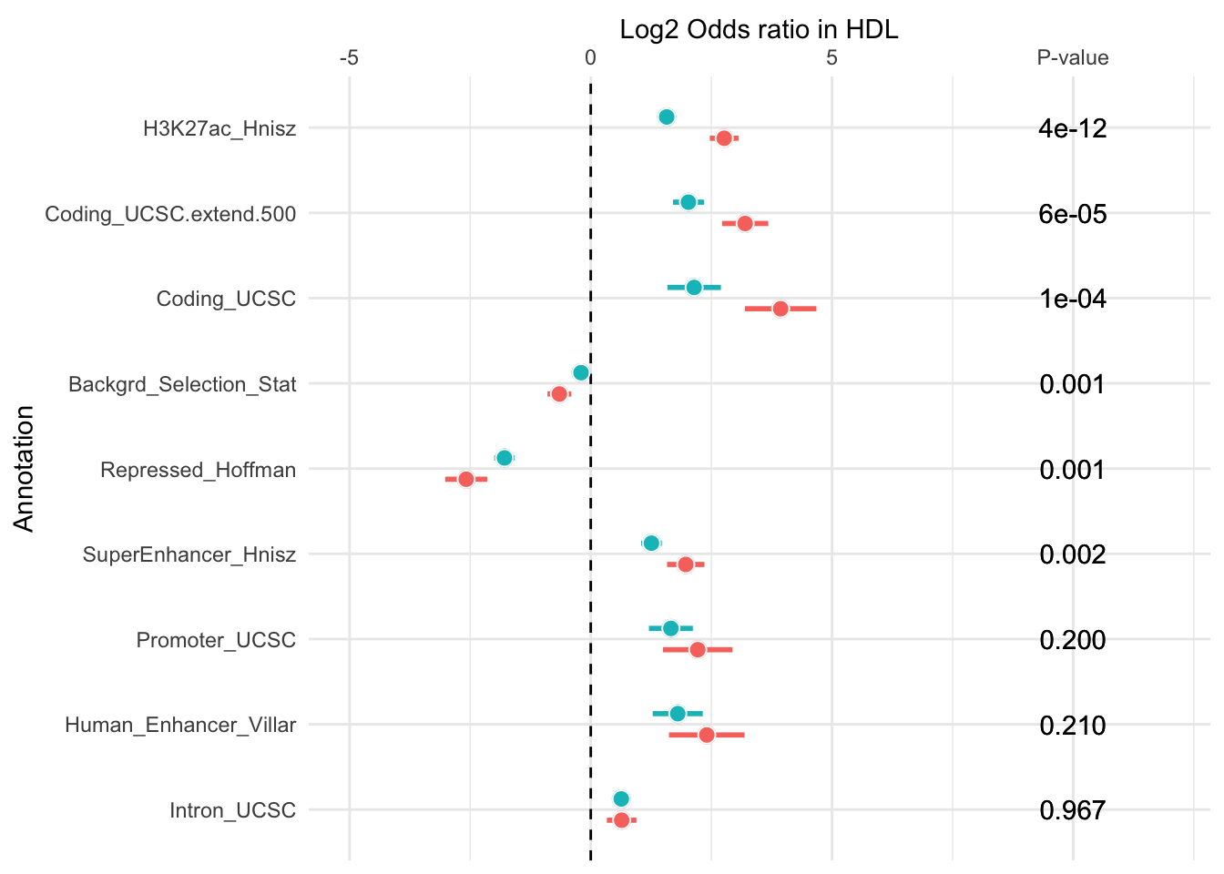
###LDL
rm(list=ls())


library('ggplot2')

mash.ldl=read.csv(("~/Downloads/mvp_complete_torus//mash/ldl.zscore.torus.merged.csv"))
mash.ldl=mash.ldl[-which(mash.ldl$annotation=="GTEx_FE_META_TISSUE_GE_MaxCPP"),]
###Orignal
raw.ldl=read.csv(("~/Downloads/mvp_complete_torus/original/original_z_mvp.ldl.zscore.torus.merged.csv"))
raw.ldl=raw.ldl[-which(raw.ldl$annotation=="GTEx_FE_META_TISSUE_GE_MaxCPP"),]


df1=mash.ldl[,c(1:4)]
colnames(df1)=c("Outcome","log2OR","Lower","Upper")
df1$se=(df1$log2OR-df1$Lower)/1.96

df2=raw.ldl[,c(1:4)]

colnames(df2)=c("Outcome","log2OR","Lower","Upper")
df2$se=(df2$log2OR-df2$Lower)/1.96

# add a group column
df1$group <- "mash"
# create a second dataset, similar format to first

# different group
df2$group <- "raw"
# and we adjust the values a bit, so it will look different in the plot
df2[,c("log2OR","Lower","Upper")]

# combine the two datasets
df = rbind(df1,df2)


z=(df1$log2OR-df2$log2OR)/sqrt(df1$se^2+df2$se^2)
p=2*pnorm(-1*abs(z))


dotCOLS = c("#a6d8f0","#f9b282")
barCOLS  <- c("#000000", "#E69F00", "#56B4E9", "#009E73", "#F0E442", "#0072B2", "#D55E00", "#CC79A7")
dotCOLS = c("blue2","red2")
barCOLS <- c("#000000", "#E69F00", "#56B4E9", "#009E73", "#F0E442", "#0072B2", "#D55E00", "#CC79A7")

df$p=c(p,p)
df$fp = format.pval(df$p,digits=1)

p = df %>% ggplot(aes(y=reorder(Outcome, desc(p)), x=log2OR, xmin=Lower, xmax=Upper, col=group, fill=group)) +
    geom_point(size=3, position=position_dodge(width = 0.5)) +
    geom_errorbarh(height=0, size=1, position=position_dodge(width = 0.5)) +
    geom_vline(xintercept=0, lty=2) +
    # geom_point(size=3, shape=21, colour="white", stroke = 0.5, position=position_dodge(width = 0.5)) +
    scale_fill_manual(values=barCOLS)+
    scale_color_manual(values=dotCOLS)+
    scale_y_discrete(name="Annotation") +
    scale_x_continuous(name="Log2 Odds ratio in ldl", limits = c(-5, 12), breaks=c(-5,0,5,10), labels=c(-5,0,5,"P-value"), position='top') +
    theme_minimal() +
    theme(legend.position=c(0.05,0.05), legend.justification=c(0,0), legend.title=element_blank()) +
    geom_text(aes(x=10, y=Outcome, label=fp), hjust=0.5, color='black')


p
###TG
rm(list=ls())
library('ggplot2')

mash.tg=read.csv(("~/Downloads/mvp_complete_torus//mash/tg.zscore.torus.merged.csv"))
mash.tg=mash.tg[-which(mash.tg$annotation=="GTEx_FE_META_TISSUE_GE_MaxCPP"),]
###Orignal
raw.tg=read.csv(("~/Downloads/mvp_complete_torus/original/original_z_mvp.tg.zscore.torus.merged.csv"))
raw.tg=raw.tg[-which(raw.tg$annotation=="GTEx_FE_META_TISSUE_GE_MaxCPP"),]


df1=mash.tg[,c(1:4)]
colnames(df1)=c("Outcome","log2OR","Lower","Upper")
df1$se=(df1$log2OR-df1$Lower)/1.96

df2=raw.tg[,c(1:4)]

colnames(df2)=c("Outcome","log2OR","Lower","Upper")
df2$se=(df2$log2OR-df2$Lower)/1.96

# add a group column
df1$group <- "mash"
# create a second dataset, similar format to first

# different group
df2$group <- "raw"
# and we adjust the values a bit, so it will look different in the plot
df2[,c("log2OR","Lower","Upper")]

# combine the two datasets
df = rbind(df1,df2)


z=(df1$log2OR-df2$log2OR)/sqrt(df1$se^2+df2$se^2)
p=2*pnorm(-1*abs(z))


dotCOLS = c("#a6d8f0","#f9b282")
barCOLS = c("#008fd5","#de6b35")
dotCOLS = c("#a6d8f0","gray80")
barCOLS = c("#008fd5","gray80")

df$p=c(p,p)
df$fp = format.pval(df$p,digits=1)

p = df %>% ggplot(aes(y=reorder(Outcome, desc(p)), x=log2OR, xmin=Lower, xmax=Upper, col=group, fill=group)) +
    geom_point(size=3, position=position_dodge(width = 0.5)) +
    geom_errorbarh(height=0, size=1, position=position_dodge(width = 0.5)) +
    geom_vline(xintercept=0, lty=2) +
    # geom_point(size=3, shape=21, colour="white", stroke = 0.5, position=position_dodge(width = 0.5)) +
    scale_fill_manual(values=barCOLS)+
    scale_color_manual(values=dotCOLS)+
    scale_y_discrete(name="Annotation") +
    scale_x_continuous(name="Log2 Odds ratio in tg", limits = c(-5, 12), breaks=c(-5,0,5,10), labels=c(-5,0,5,"P-value"), position='top') +
    theme_minimal() +
    theme(legend.position=c(0.05,0.05), legend.justification=c(0,0), legend.title=element_blank()) +
    geom_text(aes(x=10, y=Outcome, label=fp), hjust=0.5, color='black')


p
###TC
rm(list=ls())
library('ggplot2')

mash.tc=read.csv(("~/Downloads/mvp_complete_torus//mash/tc.zscore.torus.merged.csv"))
mash.tc=mash.tc[-which(mash.tc$annotation=="GTEx_FE_META_TISSUE_GE_MaxCPP"),]
###Orignal
raw.tc=read.csv(("~/Downloads/mvp_complete_torus/original/original_z_mvp.tc.zscore.torus.merged.csv"))
raw.tc=raw.tc[-which(raw.tc$annotation=="GTEx_FE_META_TISSUE_GE_MaxCPP"),]


df1=mash.tc[,c(1:4)]
colnames(df1)=c("Outcome","log2OR","Lower","Upper")
df1$se=(df1$log2OR-df1$Lower)/1.96

df2=raw.tc[,c(1:4)]

colnames(df2)=c("Outcome","log2OR","Lower","Upper")
df2$se=(df2$log2OR-df2$Lower)/1.96

# add a group column
df1$group <- "mash"
# create a second dataset, similar format to first

# different group
df2$group <- "raw"
# and we adjust the values a bit, so it will look different in the plot
df2[,c("log2OR","Lower","Upper")]

# combine the two datasets
df = rbind(df1,df2)


z=(df1$log2OR-df2$log2OR)/sqrt(df1$se^2+df2$se^2)
p=2*pnorm(-1*abs(z))


dotCOLS = c("#a6d8f0","#f9b282")
barCOLS = c("#008fd5","#de6b35")
dotCOLS = c("#a6d8f0","gray80")
barCOLS = c("#008fd5","gray80")

df$p=c(p,p)
df$fp = format.pval(df$p,digits=1)

p = df %>% ggplot(aes(y=reorder(Outcome, desc(p)), x=log2OR, xmin=Lower, xmax=Upper, col=group, fill=group)) +
    geom_point(size=3, position=position_dodge(width = 0.5)) +
    geom_errorbarh(height=0, size=1, position=position_dodge(width = 0.5)) +
    geom_vline(xintercept=0, lty=2) +
    # geom_point(size=3, shape=21, colour="white", stroke = 0.5, position=position_dodge(width = 0.5)) +
    scale_fill_manual(values=barCOLS)+
    scale_color_manual(values=dotCOLS)+
    scale_y_discrete(name="Annotation") +
    scale_x_continuous(name="Log2 Odds ratio in tc", limits = c(-5, 12), breaks=c(-5,0,5,10), labels=c(-5,0,5,"P-value"), position='top') +
    theme_minimal() +
    theme(legend.position=c(0.05,0.05), legend.justification=c(0,0), legend.title=element_blank()) +
    geom_text(aes(x=10, y=Outcome, label=fp), hjust=0.5, color='black')


p
sessionInfo()R version 4.0.2 (2020-06-22)
Platform: x86_64-apple-darwin17.0 (64-bit)
Running under: macOS 10.16
Matrix products: default
BLAS: /Library/Frameworks/R.framework/Versions/4.0/Resources/lib/libRblas.dylib
LAPACK: /Library/Frameworks/R.framework/Versions/4.0/Resources/lib/libRlapack.dylib
locale:
[1] en_US.UTF-8/en_US.UTF-8/en_US.UTF-8/C/en_US.UTF-8/en_US.UTF-8
attached base packages:
[1] stats graphics grDevices utils datasets methods base
other attached packages:
[1] forcats_0.5.1 stringr_1.4.0 dplyr_1.0.7 purrr_0.3.4
[5] readr_2.1.0 tidyr_1.1.4 tibble_3.1.6 tidyverse_1.3.1
[9] ggplot2_3.3.5
loaded via a namespace (and not attached):
[1] Rcpp_1.0.7 lubridate_1.8.0 assertthat_0.2.1 rprojroot_2.0.2
[5] digest_0.6.28 utf8_1.2.2 R6_2.5.1 cellranger_1.1.0
[9] backports_1.4.0 reprex_2.0.1 evaluate_0.14 highr_0.9
[13] httr_1.4.2 pillar_1.6.4 rlang_0.4.12 readxl_1.3.1
[17] rstudioapi_0.13 whisker_0.4 jquerylib_0.1.4 rmarkdown_2.11
[21] munsell_0.5.0 broom_0.7.10 compiler_4.0.2 httpuv_1.6.3
[25] modelr_0.1.8 xfun_0.28 pkgconfig_2.0.3 htmltools_0.5.2
[29] tidyselect_1.1.1 workflowr_1.6.2 fansi_0.5.0 crayon_1.4.2
[33] tzdb_0.2.0 dbplyr_2.1.1 withr_2.4.2 later_1.3.0
[37] grid_4.0.2 jsonlite_1.7.2 gtable_0.3.0 lifecycle_1.0.1
[41] DBI_1.1.1 git2r_0.29.0 magrittr_2.0.1 scales_1.1.1
[45] cli_3.1.0 stringi_1.7.5 farver_2.1.0 fs_1.5.0
[49] promises_1.2.0.1 xml2_1.3.2 bslib_0.3.1 ellipsis_0.3.2
[53] generics_0.1.1 vctrs_0.3.8 tools_4.0.2 glue_1.5.0
[57] hms_1.1.1 fastmap_1.1.0 yaml_2.2.1 colorspace_2.0-2
[61] rvest_1.0.2 knitr_1.36 haven_2.4.3 sass_0.4.0